2.6-kW bearingless SyRM, current-based force control#

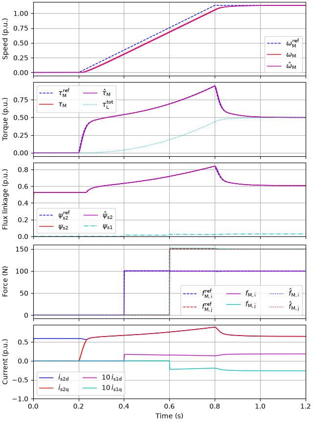
This example simulates current-based radial force control of a 2.6-kW six-phase bearingless synchronous reluctance machine (SyRM) drive, in the same operating sequence as in the direct force control example. The four-pole plane is controlled by the sensorless current-vector controller of motulator, configured with the parameters of the equivalent three-phase machine. The radial force reference is converted to the current reference of the two-pole plane using the linear force model [1], and the current is controlled in the coordinates of the vector controller. This is the classical approach to bearingless control [2], in which the force is controlled via the currents instead of directly. The machine and the controller use the same constant parameters.

from math import pi

import numpy as np

from motulator_bearingless import control, model, utils

Compute base values based on the nominal values (just for figures).

nom = utils.NominalValues(U=220, I=12, f=50, P=2.6e3, tau=14.5)
base = utils.BaseValues.from_nominal(nom, n_p=2)

Configure the system model, see the direct force control example.

par = model.BearinglessSynchronousMachinePars(
    R_s=0.215, L_1=0.03, L_d=0.03, L_q=0.01, m_d=10.0, m_q=0.2
)
machine = model.BearinglessSynchronousMachine(par)
w_M_rated = 2 * pi * 1700 / 60
k = nom.tau / w_M_rated**2  # Quadratic load torque, rated torque at the rated speed
mechanics = model.MechanicalSystem(J=0.05, B_L=lambda w_M: k * abs(w_M))
radial = model.ExternalRotorPosition()
converter = model.MultiThreePhaseConverter(u_dc=540)
mdl = model.BearinglessDrive(machine, mechanics, radial, converter)

Configure the control system. The vector controller of the four-pole plane uses the parameters of the equivalent three-phase machine, whose current is the sum of the set currents, i.e., twice the current of the four-pole plane. The minimum flux is the bias flux needed for the force production. The force controller limits the current of the two-pole plane.

par_s2 = utils.fourpole_pars(par)
cfg = control.CurrentVectorControllerCfg(
    i_s_max=2 * 1.5 * base.i,
    psi_s_min=0.3,
    alpha_c=2 * pi * 200,
    sensorless=True,
    T_s=125e-6,
)
vector_ctrl = control.CurrentVectorController(par_s2, cfg)
force_ctrl = control.CurrentBasedForceController(
    par, alpha_c=2 * pi * 200, i_s1_max=0.5 * base.i
)
speed_ctrl = control.SpeedController(J=0.05, alpha_s=2 * pi * 4)
ctrl = control.CurrentBasedForceControlSystem(vector_ctrl, force_ctrl, speed_ctrl)

Set the speed and force references as in the direct force control example.

ctrl.set_speed_ref(lambda t: min(max(t - 0.2, 0) / 0.6, 1) * w_M_rated)
ctrl.set_force_ref(lambda t: (t > 0.4) * 100 + 1j * (t > 0.6) * 150)

Create the simulation object, simulate, and plot the results. The two-pole current is shown in the coordinates of the vector controller, where it is constant in the steady state.

sim = model.Simulation(mdl, ctrl)
res = sim.simulate(t_stop=1.2)
i_lims = (-1.0, 0.95)  # Room for the legends
utils.plot(res, base, y_lims=[None, None, None, None, i_lims])

Plot the force steps. At a constant four-pole current, the force is proportional to the two-pole current, so that it follows its reference with the dynamics of the current control of the two-pole plane.

y_lims = [(-20.0, 260.0), i_lims]  # Room for the legends
utils.plot(res, base, ["force", "current"], t_lims=(0.35, 0.65), y_lims=y_lims)
print("Force at the end (N):", np.round(res.mdl.machine.f_M_ab[-1], 1))

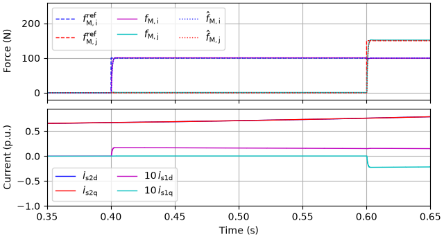
Force at the end (N): (100+150j)

References

Total running time of the script: (0 minutes 18.069 seconds)

Gallery generated by Sphinx-Gallery