2.6-kW bearingless SyRM, GradNet magnetic maps

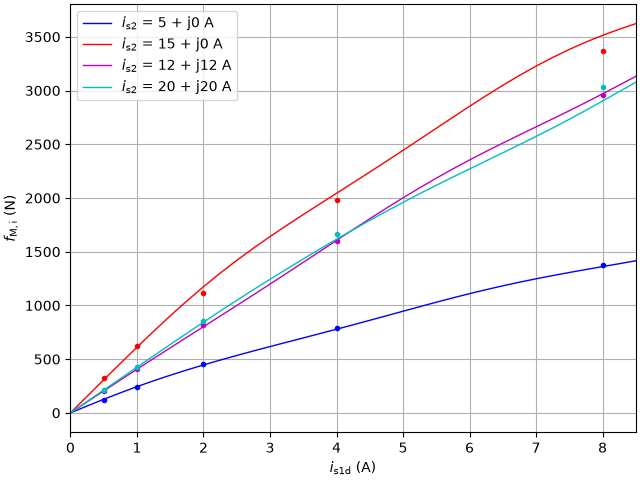
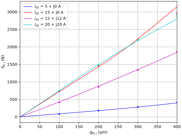
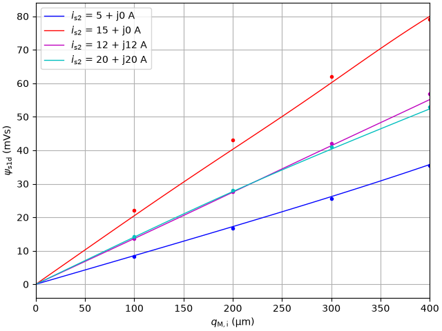
This example visualizes the GradNet magnetic maps [1] of a 2.6-kW six-phase bearingless synchronous reluctance machine (SyRM), trained on finite-element data. As in motulator, the machine model uses the energy-based current map, with or without the spatial harmonics, and the control system uses the co-energy-based flux map without the rotor angle, which approximates the average over the angle [2]. In the figures, the markers show the finite-element results, averaged over the rotor angle unless otherwise noted, and the lines show the networks. The markers are not used in the training.

from pathlib import Path
from typing import cast

import matplotlib.pyplot as plt
import numpy as np
from mpl_toolkits.mplot3d import Axes3D

import motulator_bearingless.gradnet as gn
from motulator_bearingless import model, utils

Load the dataset and the networks.

p = Path(__file__).resolve().parent if "__file__" in globals() else Path.cwd()
R_s = 0.215  # Stator resistance from [#Das2026]_
path = "trained_models/bsyrm_fem_curr_map_harm_softmax_d128.npz"
harm_map = gn.CurrentMapWithHarmonics(gn.load_gradnet(p / path))
path = "trained_models/bsyrm_fem_curr_map_softmax_d64.npz"
current_map = gn.CurrentMap(gn.load_gradnet(p / path))
path = "trained_models/bsyrm_fem_flux_map_softmax_d128.npz"
est_par = model.SaturatedBearinglessSynchronousMachinePars(
    R_s, psi_s_fcn=gn.FluxMap(gn.load_gradnet(p / path))
)
data = dict(np.load(p / "datasets" / "bsyrm_fem.npz"))
utils.set_style()


def averaged(sel: np.ndarray, *keys: str) -> dict[str, np.ndarray]:
    """Average the given signals over the rotor angle, the points being grouped."""
    keys_in = ("i_s1", "i_s2", "q_M")
    arr = np.stack([np.round(data[k][sel], 9) for k in keys_in], axis=-1)
    uniq, inv = np.unique(arr, axis=0, return_inverse=True)
    out = {k: uniq[:, m] for m, k in enumerate(keys_in)}
    for key in keys:
        vals = data[key][sel]
        out[key] = np.array([np.mean(vals[inv == n]) for n in range(len(uniq))])
    return out

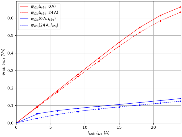
Current map of the machine model: the four-pole flux linkage versus the four-pole current at a centric rotor without the two-pole current. The lines are the currents given by the network at the finite-element flux linkages.

fem = averaged(data["set"] == 2, "psi_s1", "psi_s2")
_, i_2, _ = current_map(fem["psi_s1"], fem["psi_s2"], fem["q_M"])
i_d, i_q = np.real(fem["i_s2"]), np.imag(fem["i_s2"])
psi_d, psi_q = np.real(fem["psi_s2"]), np.imag(fem["psi_s2"])
fig, ax = plt.subplots()
for level, ls in ((0, "-"), (24, "--")):
    m = np.isclose(i_q, level) & (i_d <= 24)
    ax.plot(i_d[m], psi_d[m], ".", c="r")
    label = rf"$\psi_\mathrm{{s2d}}(i_\mathrm{{s2d}}, {level}\,\mathrm{{A}})$"
    ax.plot(np.real(i_2)[m], psi_d[m], ls, c="r", label=label)
for level, ls in ((0, "-"), (24, "--")):
    m = np.isclose(i_d, level) & (i_q <= 24)
    ax.plot(i_q[m], psi_q[m], ".", c="b")
    label = rf"$\psi_\mathrm{{s2q}}({level}\,\mathrm{{A}}, i_\mathrm{{s2q}})$"
    ax.plot(np.imag(i_2)[m], psi_q[m], ls, c="b", label=label)
ax.set_xlim(0, 24)
ax.set_ylim(0, None)
ax.set_xlabel(r"$i_\mathrm{s2d}$, $i_\mathrm{s2q}$ (A)")
ax.set_ylabel(r"$\psi_\mathrm{s2d}$, $\psi_\mathrm{s2q}$ (Vs)")
ax.legend()
plt.show()

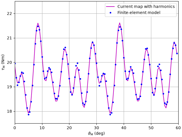
Current map with the spatial harmonics: the torque versus the rotor angle at the rated peak current, evaluated at the finite-element flux linkages. The finite-element results are not averaged here.

sel = data["set"] == 5
theta, i_1, q_M = data["theta_M"][sel], data["i_s1"][sel], data["q_M"][sel]
psi_1, psi_2 = data["psi_s1"][sel], data["psi_s2"][sel]
_, _, f_h, tau_h = harm_map(psi_1, psi_2, q_M, np.exp(1j * theta))
_, _, f_a = current_map(psi_1, psi_2, q_M)
deg = np.rad2deg(theta)

m = np.isclose(i_1, 0) & np.isclose(q_M, 0)
fig, ax = plt.subplots()
ax.plot(deg[m], tau_h[m], c="m", lw=1.5, label="Current map with harmonics")
ax.plot(deg[m], data["tau_M"][sel][m], ".", c="b", label="Finite-element model")
ax.set_xlim(0, 60)
ax.set_xticks(np.arange(0, 61, 10))
ax.set_ylim(17.5, 22.5)
ax.set_xlabel(r"$\vartheta_\mathrm{M}$ (deg)")
ax.set_ylabel(r"$\tau_\mathrm{M}$ (Nm)")
ax.legend()
plt.show()

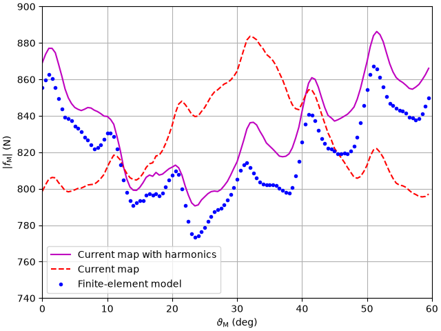
The magnitude of the radial force at i_s1 = 2 A. The force ripple appears when the two-pole current produces the force. The current map without the harmonics gives the average.

m = np.isclose(i_1, 2)
fig, ax = plt.subplots()
ax.plot(deg[m], np.abs(f_h[m]), c="m", lw=1.5, label="Current map with harmonics")
ax.plot(deg[m], np.abs(f_a[m]), "--", c="r", lw=1.5, label="Current map")
ax.plot(deg[m], np.abs(data["f_M"][sel][m]), ".", c="b", label="Finite-element model")
ax.set_xlim(0, 60)
ax.set_xticks(np.arange(0, 61, 10))
ax.set_ylim(740, 900)
ax.set_xlabel(r"$\vartheta_\mathrm{M}$ (deg)")
ax.set_ylabel(r"$|f_\mathrm{M}|$ (N)")
ax.legend()
plt.show()

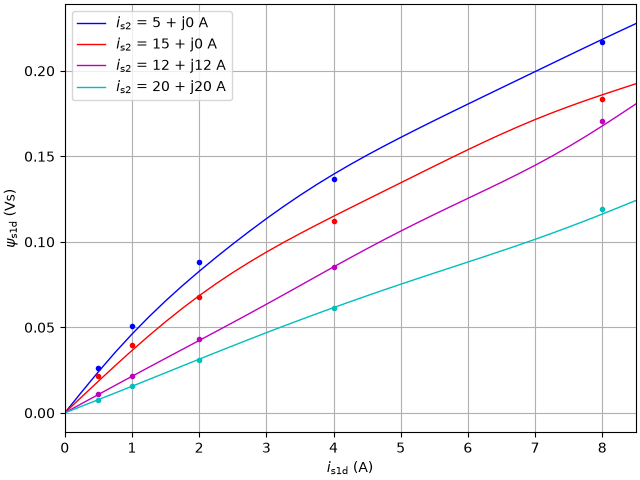
Flux map of the control system: the two-pole flux linkage versus the two-pole current at a centric rotor, for different four-pole currents.

ops = (5 + 0j, 15 + 0j, 12 + 12j, 20 + 20j)
colors = ("b", "r", "m", "c")
labels = [rf"$i_\mathrm{{s2}}$ = {i.real:.0f} + j{i.imag:.0f} A" for i in ops]
fem = averaged(data["set"] == 3, "psi_s1", "f_M")
i_1d = np.linspace(0, 8.5, 35)
i_1 = i_1d + 0j
zeros = np.zeros_like(i_1)
psi_1 = [est_par.psi_s(i_1, i_2 + zeros, zeros)[0] for i_2 in ops]
f = [est_par.f_M(i_1, i_2 + zeros, zeros) for i_2 in ops]
fem_masks = [
    np.isclose(fem["i_s2"], i_2) & np.isclose(np.imag(fem["i_s1"]), 0) for i_2 in ops
]

fig, ax = plt.subplots()
for m, psi, c, label in zip(fem_masks, psi_1, colors, labels, strict=True):
    ax.plot(np.real(fem["i_s1"][m]), np.real(fem["psi_s1"][m]), ".", c=c)
    ax.plot(i_1d, np.real(psi), c=c, label=label)
ax.set_xlim(0, 8.5)
ax.set_xlabel(r"$i_\mathrm{s1d}$ (A)")
ax.set_ylabel(r"$\psi_\mathrm{s1d}$ (Vs)")
ax.legend()
plt.show()

The radial force versus the two-pole current. The force depends nearly linearly on the two-pole current, while its slope depends strongly on the four-pole current.

fig, ax = plt.subplots()
for m, f_i, c, label in zip(fem_masks, f, colors, labels, strict=True):
    ax.plot(np.real(fem["i_s1"][m]), np.real(fem["f_M"][m]), ".", c=c)
    ax.plot(i_1d, np.real(f_i), c=c, label=label)
ax.set_xlim(0, 8.5)
ax.set_xlabel(r"$i_\mathrm{s1d}$ (A)")
ax.set_ylabel(r"$f_\mathrm{M,i}$ (N)")
ax.legend()
plt.show()

Flux map: the unbalanced magnetic pull versus the displacement, without the two-pole current. The force is in the direction of the displacement.

fem = averaged(data["set"] == 4, "psi_s1", "f_M")
q_i = np.linspace(0, 400e-6, 41)
q = q_i + 0j
zeros = np.zeros_like(q)
f = [est_par.f_M(zeros, i_2 + zeros, q) for i_2 in ops]
psi_1 = [est_par.psi_s(zeros, i_2 + zeros, q)[0] for i_2 in ops]
fem_masks = [
    np.isclose(fem["i_s2"], i_2) & np.isclose(np.imag(fem["q_M"]), 0) for i_2 in ops
]

fig, ax = plt.subplots()
for m, f_i, c, label in zip(fem_masks, f, colors, labels, strict=True):
    ax.plot(1e6 * np.real(fem["q_M"][m]), np.real(fem["f_M"][m]), ".", c=c)
    ax.plot(1e6 * q_i, np.real(f_i), c=c, label=label)
ax.set_xlim(0, 400)
ax.set_xlabel(r"$q_\mathrm{M,i}$ (µm)")
ax.set_ylabel(r"$f_\mathrm{M,i}$ (N)")
ax.legend()
plt.show()

The two-pole flux linkage induced by the displacement.

fig, ax = plt.subplots()
for m, psi, c, label in zip(fem_masks, psi_1, colors, labels, strict=True):
    ax.plot(1e6 * np.real(fem["q_M"][m]), 1e3 * np.real(fem["psi_s1"][m]), ".", c=c)
    ax.plot(1e6 * q_i, 1e3 * np.real(psi), c=c, label=label)
ax.set_xlim(0, 400)
ax.set_xlabel(r"$q_\mathrm{M,i}$ (µm)")
ax.set_ylabel(r"$\psi_\mathrm{s1d}$ (mVs)")
ax.legend()
plt.show()

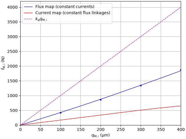
The unbalanced magnetic pull at the rated peak current, at constant currents according to the flux map and at constant flux linkages according to the current map. The flux linkages are those of the finite-element model at a centric rotor. The pull is destabilizing also at constant flux linkages, i.e., the energy is concave in the displacement. Therefore, the current map represents the shifted energy W + k_q*abs(q_M)**2/2, which is convex where k_q exceeds the stiffness of the pull at constant currents.

i_2 = 12 + 12j
fem_0 = averaged((data["set"] == 2) & np.isclose(data["i_s2"], i_2), "psi_s2")
_, _, f_psi = current_map(zeros, fem_0["psi_s2"][0] + zeros, q)
f_i = est_par.f_M(zeros, i_2 + zeros, q)
k_q = current_map.fcn.k_q * current_map.f_base / current_map.q_base
m = fem_masks[ops.index(i_2)]

fig, ax = plt.subplots()
ax.plot(1e6 * np.real(fem["q_M"][m]), np.real(fem["f_M"][m]), ".", c="b")
ax.plot(1e6 * q_i, np.real(f_i), c="b", label="Flux map (constant currents)")
ax.plot(1e6 * q_i, np.real(f_psi), c="r", label="Current map (constant flux linkages)")
ax.plot(1e6 * q_i, k_q * q_i, "--", c="m", label=r"$k_q q_\mathrm{M,i}$")
ax.set_xlim(0, 400)
ax.set_ylim(0, None)
ax.set_xlabel(r"$q_\mathrm{M,i}$ (µm)")
ax.set_ylabel(r"$f_\mathrm{M,i}$ (N)")
ax.legend()
plt.show()

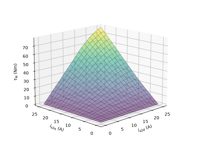
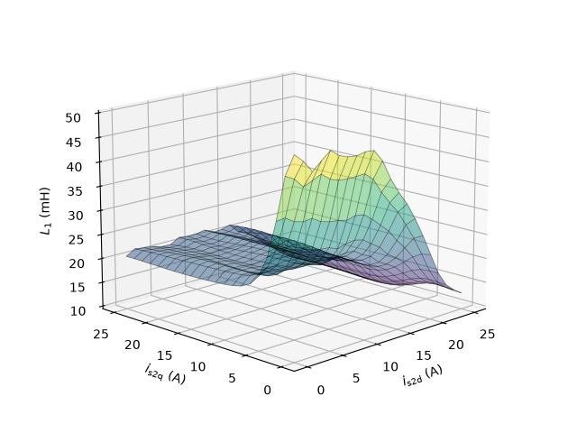
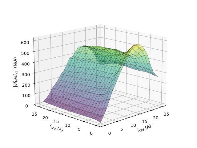
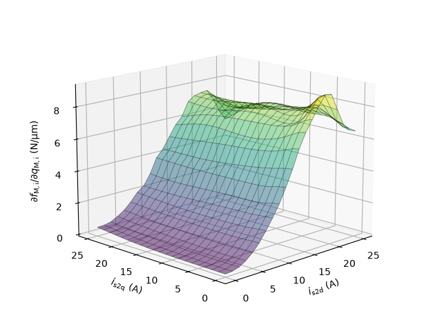
Characteristics of the flux map over the four-pole current at a centric rotor without the two-pole current: the torque, the incremental inductance of the two-pole plane, the slope of the radial force with respect to the two-pole current, and the stiffness of the unbalanced magnetic pull at constant currents. The rated peak current is 17 A.

d = np.linspace(0, 25, 21)
i_d, i_q = np.meshgrid(d, d, indexing="ij")
i_2 = np.ravel(i_d + 1j * i_q)
zeros = np.zeros_like(i_2)
_, psi_2 = est_par.psi_s(zeros, i_2, zeros)
L_s = est_par.incr_ind_mat(zeros, i_2, zeros)
eps_i, eps_q = 1e-3, 1e-6
maps = (
    (6 * np.imag(i_2 * np.conj(psi_2)), r"$\tau_\mathrm{M}$ (Nm)"),
    (1e3 * 0.5 * (L_s[:, 0, 0] + L_s[:, 1, 1]), r"$L_1$ (mH)"),
    (
        np.abs(est_par.f_M(zeros + eps_i, i_2, zeros)) / eps_i,
        r"$|\partial f_\mathrm{M}/\partial i_\mathrm{s1}|$ (N/A)",
    ),
    (
        1e-6 * np.real(est_par.f_M(zeros, i_2, zeros + eps_q)) / eps_q,
        r"$\partial f_\mathrm{M,i}/\partial q_\mathrm{M,i}$ (N/µm)",
    ),
)
for z, zlabel in maps:
    fig, ax = plt.subplots(subplot_kw={"projection": "3d"})
    ax = cast(Axes3D, ax)
    z_grid = np.reshape(z, i_d.shape)
    ax.plot_surface(i_d, i_q, z_grid, cmap="viridis", alpha=0.5)
    ax.plot_wireframe(i_d, i_q, z_grid, color="black", linewidth=0.5, alpha=0.5)
    ax.set_xlabel(r"$i_\mathrm{s2d}$ (A)")
    ax.set_ylabel(r"$i_\mathrm{s2q}$ (A)")
    ax.zaxis.set_rotate_label(False)
    ax.set_zlabel(zlabel, rotation=90)
    ax.view_init(elev=15, azim=-135)
    plt.show()

• 
• 
• 
• 

References

[1]

Li, Foissner, Martin, Piippo, Hinkkanen, “Gradient networks for universal magnetic modeling of synchronous machines,” 2026, https://arxiv.org/abs/2602.14947

[2]

Das, Martin, Kontodinas, Hinkkanen, “Direct force control of six-phase bearingless synchronous machines,” Proc. ICEM, 2026, https://doi.org/10.1109/ICEM68283.2026.11757980