Finite-Element Data#
The gradient networks of the examples are trained on the finite-element data of a 2.6-kW six-phase bearingless synchronous reluctance machine. The FEMM model, the generation of the dataset, and the training of the networks are in the folder fem/ of the repository, and the results are in examples/datasets/ and examples/trained_models/.
Machine#
The rated values and the stator resistance are from [Das et al., 2026]. Nothing has been calibrated to measurements.
Quantity |
Value |
|---|---|
Stator |
36 slots, inner radius 72.5 mm, outer radius 117.5 mm |
Winding |
Single layer, 16 conductors per slot, 48 series turns per phase |
Phases |
Six coil groups spanning \(90^\circ\), with the magnetic axes at \(60^\circ\) intervals |
Rotor |
Four poles, four streamline flux barriers per pole, 1.5-mm ribs |
Air gap, stack length, shaft radius |
1 mm, 195.25 mm, 27 mm |
Steel |
Tables of |
The end-winding leakage, the skew, the axial end effects, and the losses are not included. The solid shaft is treated as magnetostatic.
Conventions#
As in System Model, the conventions are those of [Ahmed et al., 2023] and [Das et al., 2026]:
The winding function of phase \(k\) has its maxima at \((k - 1)60^\circ\), for both the two-pole and four-pole components.
The rotor angle \(\thetaM\) is the angle of the d-axis (no barriers) from the axis of phase 1.
The space vectors of the planes \(h = 1\) and \(h = 2\) are peak-valued and in rotor coordinates, \(\ish{1} = \e^{-\jj\thetaM}\ish{1}^\mathrm{s}\) and \(\ish{2} = \e^{-2\jj\thetaM}\ish{2}^\mathrm{s}\). Hence, \(i_\mathrm{s1d}\) and \(i_\mathrm{s2d}\) together give a positive force along the i-axis at \(\thetaM = 0\).
The displacement \(\qM^\mathrm{s}\) is the position of the rotor center relative to the center of the stator bore. In FEMM, the rotor center stays at the origin and the stator moves by \(-\qM^\mathrm{s}\), so that the torque integral refers to the rotor center.
Boundary Conditions#
\(A = 0\) on the outer surface of the stator. This is the only outer boundary, since the whole cross-section is modeled and the shaft is a meshed part of the rotor (solid steel). The two-pole flux crosses the center of the rotor, so that the shaft is not a boundary of the field, unlike in one-pole models of machines without radial force. \(A = 0\) on the shaft surface and a nonmagnetic shaft are available for comparison (Params.shaft).
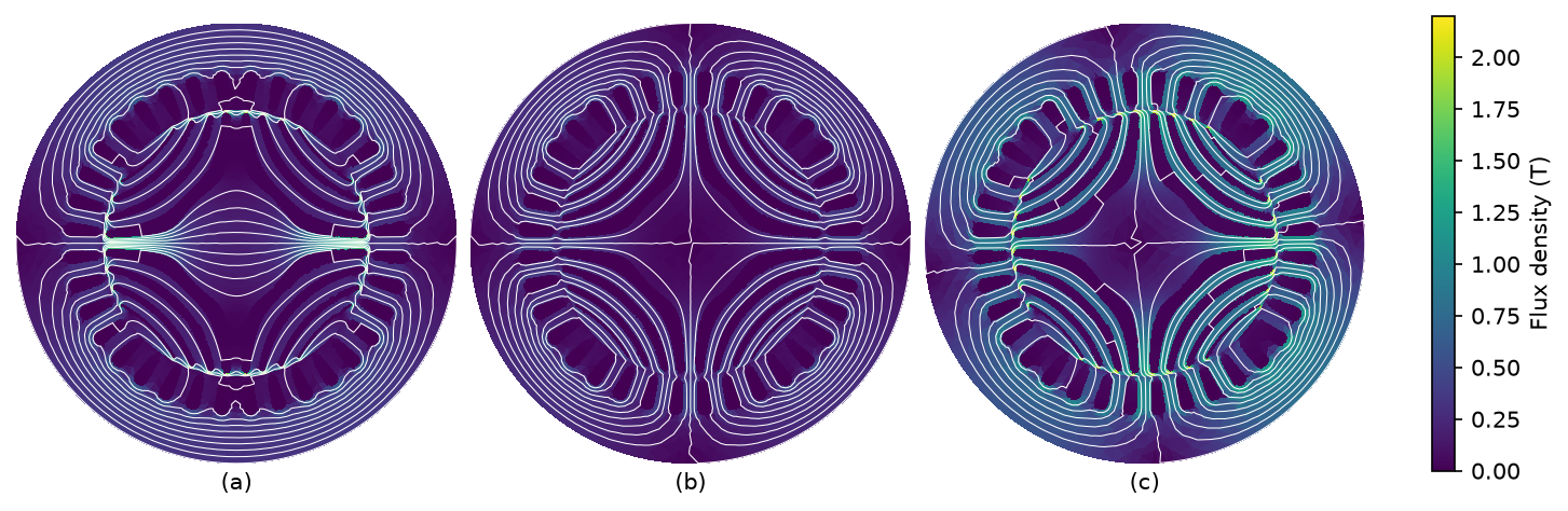
Flux lines and flux density at \(\thetaM = 0\) and a centric rotor: (a) \(\ish{1} = 5\) A and \(\ish{2} = 0\); (b) \(\ish{1} = 0\) and \(\ish{2} = 5\) A; (c) \(\ish{1} = 2\) A and \(\ish{2} = 12 + \jj 12\) A. The two-pole flux crosses the center of the rotor, and no flux crosses the outer boundary.#
Dataset#
The energy function depends on seven variables, so a tensor grid is out of the question. The points are created by sample_plan.py:
Set 0: 16384 training points from a Sobol sequence, denser at small two-pole currents and displacements. The ranges are \(|\ish{1}| \leq 15\) A, \(|\ish{2}| \leq 36\) A (the rated peak current is 17 A), \(|\qM| \leq 400\) µm, and \(0 \leq \thetaM < 60^\circ\).
Set 1: 1024 test points from another Sobol sequence in the same ranges, spread more widely. They are not used in the training.
Sets 2–5: structured slices for validation and plots, not used in the training.
Set 6: 4096 additional training points in the normal operating range, \(|\ish{1}| \leq 3\) A, \(|\ish{2}| \leq 26\) A, and \(|\qM| \leq 100\) µm.
Set 7: 1024 additional training points around no load, as set 6 but with \(0 \leq i_\mathrm{s2q} \leq 4\) A, since the two-pole inductance and the force constant change quickly with \(i_\mathrm{s2q}\) there.
The meshes have about 60 000 elements. Compared with about 730 000 elements, the differences in the checked points are at most 2.7 mVs in the flux linkages and 0.8 % in the force.
Networks#
The architecture of the networks is that of motulator: one softmax gradient network, see Gradient-Network Magnetic Maps. The machine model uses energy-based current maps and the controller a co-energy-based flux map:
File in |
Map |
Hidden units |
Periodic features \(k\) |
|---|---|---|---|
|
Current map with harmonics |
128 |
6, 36 |
|
Current map |
64 |
|
|
Flux map |
128 |
The output of the networks is averaged over the symmetry group, see Gradient-Network Magnetic Maps. One finite-element point thus informs 16 points of the input space, and the force and the two-pole flux linkage vanish exactly at \(\ish{1} = 0\) and \(\qM = 0\). The same symmetries hold for the energy as a function of the flux linkages.
At the nine points checked by central differences (check_model.py hessian), the Hessian of the co-energy is symmetric within the relative error of \(1.2\cdot 10^{-4}\) and positive definite, i.e., the co-energy is jointly convex in the currents and the displacement. The stiffness of the unbalanced magnetic pull at constant flux linkages is positive at these points, from 0.02 N/µm to 4.7 N/µm, so that the energy is locally concave in the displacement. The current maps use \(k_q = 10\) N/µm. According to the flux map, it exceeds the largest eigenvalue of the stiffness matrix of the pull at constant currents at 99.9 % of the data points, and the exceptions are at displacements above 160 µm. The networks without the rotor angle are trained on the same data, so that they approximate the average over the rotor angle. The order \(k = 36\) is added to the fundamental order \(k = 6\), since the slot harmonics of the 36-slot stator dominate the torque ripple. It decreases the torque error of the normal operating range from 0.27 Nm to 0.18 Nm.
The RMS errors on the held-out test points are given below, for all the points and for those in the normal operating range, \(|\ish{1}| < 3\) A, \(|\ish{2}| < 26\) A, and \(|\qM| < 100\) µm. The errors of the models without the rotor angle include the variation over the angle.
Map |
Points |
\(\ish{1}\) or \(\psish{1}\) |
\(\ish{2}\) or \(\psish{2}\) |
\(\fM\) |
\(\tauM\) |
|---|---|---|---|---|---|
Current map with harmonics |
All |
105 mA |
151 mA |
59 N |
0.37 Nm |
Normal |
40 mA |
97 mA |
15 N |
0.18 Nm |
|
Current map |
All |
366 mA |
384 mA |
159 N |
1.6 Nm |
Normal |
80 mA |
195 mA |
27 N |
0.76 Nm |
|
Flux map |
All |
7.6 mVs |
3.7 mVs |
198 N |
1.5 Nm |
Normal |
2.3 mVs |
2.3 mVs |
32 N |
0.69 Nm |
The mean of the force error over the rotor angle at \(|\ish{1}| \leq 2\) A is below 2 % for the current maps and about 3 % for the flux map.
Usage#
The scripts need femm-qt, the cross-platform FEMM 5.0, and its Python interface in the same environment, installed from the femm-qt checkout with pip install -e pyfemm (not the pyfemm package of FEMM 4.2), as well as the optional dependencies, pip install -e .[fem]. The Python interface finds femm_headless in the build directory of the checkout, in the directory given by FEMM_DIR, or on PATH.
python sample_plan.py plan.npz
python run_maps.py plan.npz results.txt 7          # Continues an interrupted run
python make_dataset.py plan.npz results.txt ../examples/datasets/bsyrm_fem.npz
python check_model.py boundary mesh symmetry hessian field field.png

M=../examples/trained_models
D=../examples/datasets/bsyrm_fem.npz
python train_gradnet.py $D $M/bsyrm_fem_curr_map_harm_softmax_d128.npz --map current --embed 128 --k 6 36 --seed 4
python train_gradnet.py $D $M/bsyrm_fem_curr_map_softmax_d64.npz --map current --embed 64
python train_gradnet.py $D $M/bsyrm_fem_flux_map_softmax_d128.npz --map flux --embed 128 --s_2 0.007
python evaluate_gradnet.py $D $M/bsyrm_fem_curr_map_harm_softmax_d128.npz
python compare_control.py results.json
More points can be appended to the plan: run_maps.py skips the points already solved. The temporary files of FEMM go to /dev/shm/bsyrm_femm (or set BSYRM_FEMM_WORK).
File |
Contents |
|---|---|
|
Parametric geometry, materials, winding, and the solver interface |
|
Dataset |
|
Checks of the model and field plots |
|
Training of the networks and their errors |
|
Direct force control with different machine and controller models |