Note
Go to the end to download the full example code.
5.5-kW PM-SyRM, saturated#
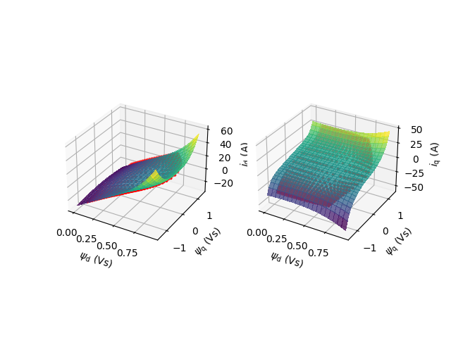
This example simulates sensorless stator-flux-vector control of a 5.5-kW PM-SyRM (Baldor ECS101M0H7EF4) drive. The machine model is parametrized using the algebraic saturation model from [1], fitted to the flux linkage maps measured using the constant-speed test. For comparison, the measured data is plotted together with the model predictions. Notice that the control system used in this example does not consider the saturation, only the system model does.
from os import path
import inspect

import numpy as np
from scipy.io import loadmat
from scipy.optimize import minimize_scalar
import matplotlib.pyplot as plt

from motulator.drive import model
import motulator.drive.control.sm as control
from motulator.drive.utils import (
    BaseValues, NominalValues, plot, Sequence, SynchronousMachinePars)
Compute base values based on the nominal values (just for figures).
nom = NominalValues(U=370, I=8.8, f=60, P=5.5e3, tau=29.2)
base = BaseValues.from_nominal(nom, n_p=2)
Create a saturation model, which will be used in the machine model in the following simulations.
# pylint: disable=too-many-locals
def i_s(psi_s):
    """
    Saturation model for a 5.5-kW PM-SyRM.

    This model takes into account the bridge saturation in addition to the
    regular self- and cross-saturation effects of the d- and q-axis. The bridge
    saturation model is based on a nonlinear reluctance element in parallel
    with the Norton-equivalent PM model.

    Parameters
    ----------
    psi_s : complex
        Stator flux linkage (Vs).

    Returns
    -------
    complex
        Stator current (A).

    Notes
    -----
    For simplicity, the saturation model parameters are hard-coded in the
    function below. This model can also be used for other PM-SyRMs by changing
    the model parameters.

    """
    # d-axis self-saturation
    a_d0, a_dd, S = 3.96, 28.46, 4
    # q-axis self-saturation
    a_q0, a_qq, T = 5.89, 2.672, 6
    # Cross-saturation
    a_dq, U, V = 41.52, 1, 1
    # PM model and bridge saturation
    a_b, a_bp, k_q, psi_n, W = 81.75, 1, .1, .804, 2

    # Inverse inductance functions for the d- and q-axis
    G_d = a_d0 + a_dd*np.abs(psi_s.real)**S + (
        a_dq/(V + 2)*np.abs(psi_s.real)**U*np.abs(psi_s.imag)**(V + 2))
    G_q = a_q0 + a_qq*np.abs(psi_s.imag)**T + (
        a_dq/(U + 2)*np.abs(psi_s.real)**(U + 2)*np.abs(psi_s.imag)**V)

    # Bridge flux
    psi_b = psi_s.real - psi_n
    # State of the bridge saturation depends also on the q-axis flux
    psi_b_sat = np.sqrt(psi_b**2 + k_q*psi_s.imag**2)
    # Inverse inductance function for the bridge saturation
    G_b = a_b*psi_b_sat**W/(1 + a_bp*psi_b_sat**W)

    # Stator current
    return G_d*psi_s.real + G_b*psi_b + 1j*(G_q + k_q*G_b)*psi_s.imag
Plot the saturation model (surfaces) and the measured flux map data (points). Notice that the simulation uses the the algebraic model only. The measured data is shown only for comparison.
# Load the measured data from the MATLAB file
p = path.dirname(path.abspath(inspect.getfile(inspect.currentframe())))
data = loadmat(p + "/ABB_400rpm_map.mat")
psi_d_meas, psi_q_meas = data["psid_map"], data["psiq_map"]
i_d_meas, i_q_meas = data["id_map"], data["iq_map"]

# Generate the data to be plotted using the algebraic saturation model
psi_d = np.arange(0, 1, .05)
psi_q = np.arange(-1.35, 1.35, .05)
psi_d, psi_q = np.meshgrid(psi_d, psi_q)
i_d, i_q = i_s(psi_d + 1j*psi_q).real, i_s(psi_d + 1j*psi_q).imag

# Create the figure and the subplots
fig = plt.figure()
ax1 = fig.add_subplot(1, 2, 1, projection="3d")
ax2 = fig.add_subplot(1, 2, 2, projection="3d")

# Plot the d-axis experimental data as points
surf1 = ax1.scatter(psi_d_meas, psi_q_meas, i_d_meas, marker=".", color="r")

# Plot the d-axis model predictions as surfaces
surf2 = ax1.plot_surface(
    psi_d, psi_q, i_d, alpha=.75, cmap="viridis", antialiased=False)
ax1.set_xlabel(r"$\psi_\mathrm{d}$ (Vs)")
ax1.set_ylabel(r"$\psi_\mathrm{q}$ (Vs)")
ax1.set_zlabel(r"$i_\mathrm{d}$ (A)")

# Plot the q-axis experimental data as points
surf3 = ax2.scatter(psi_d_meas, psi_q_meas, i_q_meas, marker=".", color="r")

# Plot the q-axis model predictions as surfaces
surf4 = ax2.plot_surface(
    psi_d, psi_q, i_q, alpha=.75, cmap="viridis", antialiased=False)
ax2.set_xlabel(r"$\psi_\mathrm{d}$ (Vs)")
ax2.set_ylabel(r"$\psi_\mathrm{q}$ (Vs)")
ax2.set_zlabel(r"$i_\mathrm{q}$ (A)")

plt.show()
Solve the PM flux linkage for the initial value of the stator flux linkage, which is needed in the machine model below.
res = minimize_scalar(
    lambda psi_d: np.abs(i_s(psi_d)), bounds=(0, base.psi), method="bounded")
psi_s0 = complex(res.x)  # psi_s0 = 0.477
Configure the system model.
mdl_par = SynchronousMachinePars(n_p=2, R_s=.63)
machine = model.SynchronousMachine(mdl_par, i_s=i_s, psi_s0=psi_s0)
# Magnetically linear PM-SyRM model for comparison
# mdl_par = SynchronousMachinePars(
#     n_p=2, R_s=.63, L_d=18e-3, L_q=110e-3, psi_f=.47)
# machine = model.SynchronousMachine(mdl_par)
mechanics = model.StiffMechanicalSystem(J=.015)
converter = model.VoltageSourceConverter(u_dc=540)
mdl = model.Drive(converter, machine, mechanics)
Configure the control system.
# Control system is based on the constant inductances
par = SynchronousMachinePars(n_p=2, R_s=.63, L_d=18e-3, L_q=110e-3, psi_f=.47)
# Limit the maximum reference flux to the base value
cfg = control.FluxTorqueReferenceCfg(
    par, max_i_s=2*base.i, k_u=1, max_psi_s=base.psi)
ctrl = control.FluxVectorControl(par, cfg, J=.015, sensorless=True)
# Select a lower speed-estimation bandwidth to mitigate the saturation effects
ctrl.observer = control.Observer(
    control.ObserverCfg(par, alpha_o=2*np.pi*40, sensorless=True))
Set the speed reference and the external load torque.
# Speed reference (electrical rad/s)
times = np.array([0, .125, .25, .375, .5, .625, .75, .875, 1])*4
values = np.array([0, 0, 1, 1, 0, -1, -1, 0, 0])*base.w
ctrl.ref.w_m = Sequence(times, values)
# External load torque
times = np.array([0, .125, .125, .875, .875, 1])*4
values = np.array([0, 0, 1, 1, 0, 0])*nom.tau
mdl.mechanics.tau_L = Sequence(times, values)
Create the simulation object and simulate it.
sim = model.Simulation(mdl, ctrl)
sim.simulate(t_stop=4)
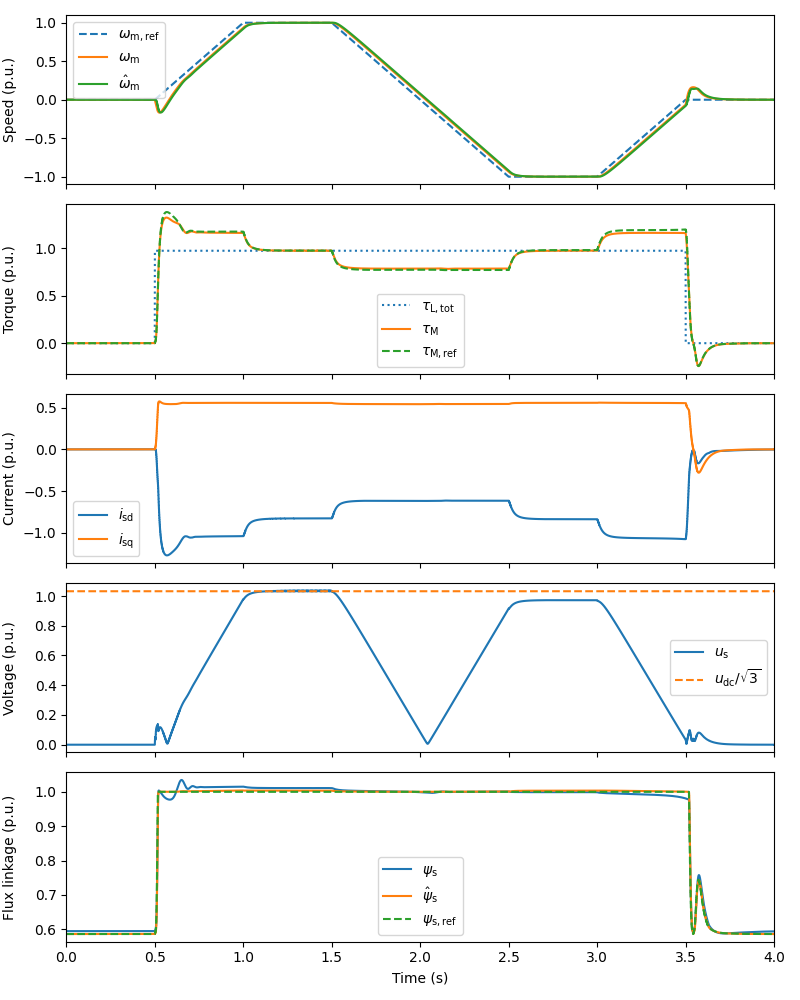
Plot results in per-unit values.
plot(sim, base)
References
Total running time of the script: (0 minutes 15.939 seconds)