6.7-kW SyRM

This example simulates sensorless vector control of a 6.7-kW SyRM drive. Square-wave signal injection is used with a simple phase-locked loop.

import numpy as np
import matplotlib.pyplot as plt

from motulator.drive import model
import motulator.drive.control.sm as control
from motulator.drive.utils import (
    BaseValues, NominalValues, plot, Sequence, SynchronousMachinePars)

Compute base values based on the nominal values (just for figures).

nom = NominalValues(U=370, I=15.5, f=105.8, P=6.7e3, tau=20.1)
base = BaseValues.from_nominal(nom, n_p=2)

Configure the system model.

mdl_par = SynchronousMachinePars(
    n_p=2, R_s=.54, L_d=41.5e-3, L_q=6.2e-3, psi_f=0)
machine = model.SynchronousMachine(mdl_par)
mechanics = model.StiffMechanicalSystem(J=.015)
converter = model.Inverter(u_dc=540)
mdl = model.Drive(converter, machine, mechanics)

Configure the control system.

par = mdl_par  # Assume accurate machine model parameter estimates
cfg = control.CurrentReferenceCfg(
    par, nom_w_m=base.w, max_i_s=2*base.i, min_psi_s=.5*base.psi)
ctrl = control.SignalInjectionControl(par, cfg, J=.015, T_s=250e-6)
# ctrl.current_ctrl = control.sm.CurrentControl(par, 2*np.pi*100)
# ctrl.signal_inj = control.sm.SignalInjection(par, U_inj=200)

Set the speed reference and the external load torque.

# Speed reference
times = np.array([0, .25, .25, .375, .5, .625, .75, .75, 1])*4
values = np.array([0, 0, 1, 1, 0, -1, -1, 0, 0])*.1*base.w
ctrl.ref.w_m = Sequence(times, values)
# External load torque
times = np.array([0, .125, .125, .875, .875, 1])*4
values = np.array([0, 0, 1, 1, 0, 0])*nom.tau
mdl.mechanics.tau_L = Sequence(times, values)

Create the simulation object and simulate it.

sim = model.Simulation(mdl, ctrl)
sim.simulate(t_stop=4)

Plot results in per-unit values.

# Plot the "basic" figure
plot(sim, base)

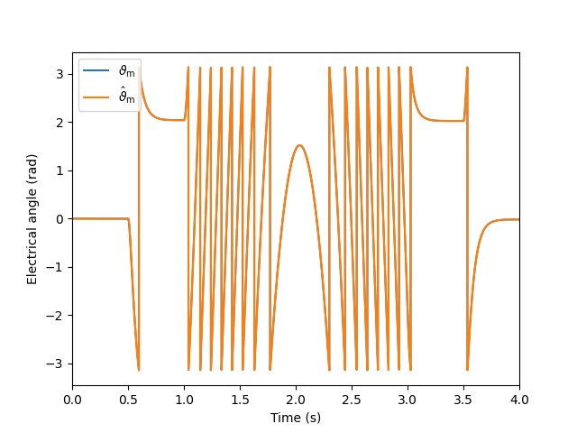
# Plot also the angles
mdl = sim.mdl  # Continuous-time data
ctrl = sim.ctrl.data  # Discrete-time data
ctrl.t = ctrl.ref.t  # Discrete time
plt.figure()
plt.plot(
    mdl.machine.data.t,
    mdl.machine.data.theta_m,
    label=r"$\vartheta_\mathrm{m}$")
plt.plot(
    ctrl.t,
    ctrl.fbk.theta_m,
    ds="steps-post",
    label=r"$\hat \vartheta_\mathrm{m}$")
plt.legend()
plt.xlim(0, 4)
plt.xlabel("Time (s)")
plt.ylabel("Electrical angle (rad)")
plt.show()

• 
•