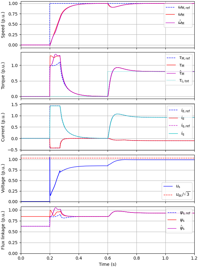
2.2-kW PMSM, with PM flux adaptation#

This example simulates sensorless current-vector control of a 2.2-kW PMSM drive. The PM-flux adaptation is enabled [1]. To demonstrate adaptation, the initial value of the PM-flux estimate has an error of 25%.

from math import pi

import matplotlib.pyplot as plt

import motulator.drive.control.sm as control
from motulator.drive import model, utils

Compute base values based on the nominal values (just for figures).

nom = utils.NominalValues(U=370, I=4.3, f=75, P=2.2e3, tau=14)
base = utils.BaseValues.from_nominal(nom, n_p=3)

Configure the system model.

par = model.SynchronousMachinePars(n_p=3, R_s=3.6, L_d=0.036, L_q=0.051, psi_f=0.545)
machine = model.SynchronousMachine(par)
mechanics = model.MechanicalSystem(J=0.015)
converter = model.VoltageSourceConverter(u_dc=540)
mdl = model.Drive(machine, mechanics, converter)

Configure the control system.

# PM-flux estimate is about 75% of the actual value
est_par = model.SynchronousMachinePars(n_p=3, R_s=3.6, L_d=0.036, L_q=0.051, psi_f=0.4)
# Gain `k_f` enables the PM-flux disturbance estimation at speeds above 0.2 p.u.
cfg = control.CurrentVectorControllerCfg(
    i_s_max=1.5 * base.i, k_f=lambda w_m: max(0.05 * (abs(w_m) - 0.2 * base.w), 0)
)
vector_ctrl = control.CurrentVectorController(est_par, cfg)
speed_ctrl = control.SpeedController(J=0.015, alpha_s=2 * pi * 4)
ctrl = control.VectorControlSystem(vector_ctrl, speed_ctrl)

Set the speed reference and the external load torque.

ctrl.set_speed_ref(lambda t: (t > 0.2) * 1 * base.w_M)
mdl.mechanics.set_external_load_torque(lambda t: (t > 0.6) * nom.tau)

Create the simulation object, simulate, and plot the results in per-unit values.

sim = model.Simulation(mdl, ctrl)
res = sim.simulate(t_stop=1.2)
utils.plot(res, base)

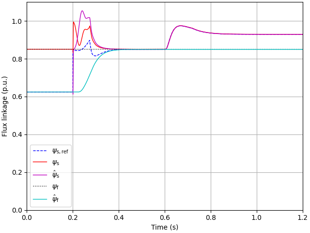
Plot the actual and estimated values for flux linkages.

plt.figure()
plt.plot(
    res.ctrl.t, res.ctrl.ref.psi_s / base.psi, "--", label=r"$\psi_\mathrm{s,ref}$"
)
plt.plot(
    res.mdl.t, abs(res.mdl.machine.psi_s_dq) / base.psi, label=r"$\psi_\mathrm{s}$"
)
plt.plot(
    res.ctrl.t, abs(res.ctrl.fbk.psi_s) / base.psi, label=r"$\hat{\psi}_\mathrm{s}$"
)
plt.axhline(0.545 / base.psi, color="k", linestyle=":", label=r"$\psi_\mathrm{f}$")
plt.plot(res.ctrl.t, res.ctrl.fbk.psi_f / base.psi, label=r"$\hat{\psi}_\mathrm{f}$")
plt.xlabel("Time (s)")
plt.ylabel("Flux linkage (p.u.)")
plt.legend()
plt.xlim(0, 1.2)
plt.ylim(0, 1.1)

plt.show()

References

Total running time of the script: (0 minutes 6.960 seconds)

Gallery generated by Sphinx-Gallery