Note
Go to the end to download the full example code.
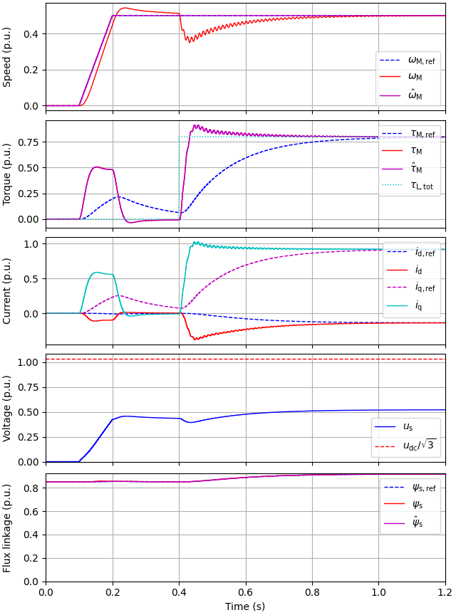
2.2-kW PMSM, 2-mass mechanics#
This example simulates observer-based V/Hz control of a 2.2-kW PMSM drive. The mechanical subsystem is modeled as a two-mass system. The resonance frequency of the mechanics is around 85 Hz. The mechanical parameters correspond to [1], except that the torsional damping is set to a smaller value in this example.
import matplotlib.pyplot as plt
import numpy as np

import motulator.drive.control.sm as control
from motulator.drive import model, utils
Compute base values from the nominal values.
nom = utils.NominalValues(U=370, I=4.3, f=75, P=2.2e3, tau=14)
base = utils.BaseValues.from_nominal(nom, n_p=3)
Configure the system model.
par = model.SynchronousMachinePars(n_p=3, R_s=3.6, L_d=0.036, L_q=0.051, psi_f=0.545)
machine = model.SynchronousMachine(par)
mechanics = model.TwoMassMechanicalSystem(J_M=0.005, J_L=0.005, K_S=700, C_S=0.01)
converter = model.VoltageSourceConverter(u_dc=540)
mdl = model.Drive(machine, mechanics, converter)
Configure the control system.
est_par = par  # Assume accurate model parameter estimates
cfg = control.ObserverBasedVHzControllerCfg(i_s_max=1.5 * base.i)
vhz_ctrl = control.ObserverBasedVHzController(est_par, cfg)
ctrl = control.VHzControlSystem(vhz_ctrl)
Set the speed reference and the external load torque.
# Speed reference
times = np.array([0, 0.1, 0.2, 1])
values = np.array([0, 0, 1, 1]) * 0.5 * base.w_M
ctrl.set_speed_ref(utils.SequenceGenerator(times, values))
# External load torque
times = np.array([0, 0.4, 0.4, 1])
values = np.array([0, 0, 1, 1]) * nom.tau
mdl.mechanics.set_external_load_torque(utils.SequenceGenerator(times, values))
Create the simulation object, simulate, and plot the results in per-unit values.
sim = model.Simulation(mdl, ctrl)
res = sim.simulate(t_stop=1.2)
# sphinx_gallery_thumbnail_number = 3
utils.plot(res, base)
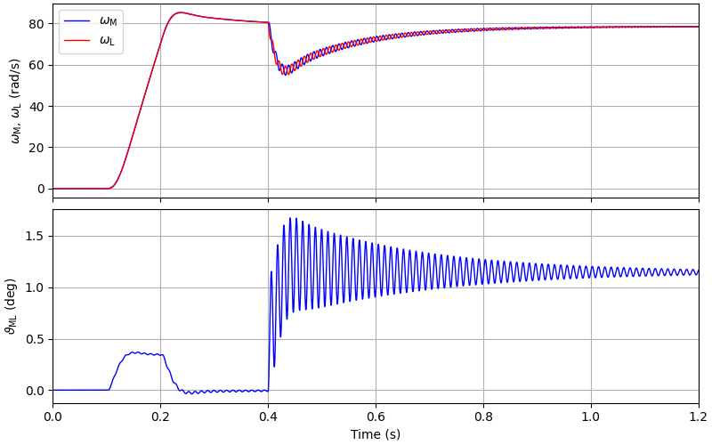
Plot the load speed and the twist angle.
t_lims = (0, 1.2)
_, (ax1, ax2) = plt.subplots(2, 1, figsize=(8, 5))
ax1.plot(res.mdl.t, res.mdl.mechanics.w_M, label=r"$\omega_\mathrm{M}$")
ax1.plot(res.mdl.t, res.mdl.mechanics.w_L, label=r"$\omega_\mathrm{L}$")
ax2.plot(res.mdl.t, res.mdl.mechanics.theta_ML * 180 / np.pi)
ax1.set_xlim(t_lims)
ax2.set_xlim(t_lims)
ax1.set_xticklabels([])
ax1.legend()
ax1.set_ylabel(r"$\omega_\mathrm{M}$, $\omega_\mathrm{L}$ (rad/s)")
ax2.set_ylabel(r"$\vartheta_\mathrm{ML}$ (deg)")
ax2.set_xlabel("Time (s)")
plt.show()
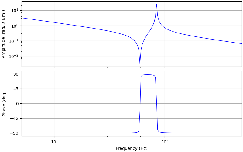
Plot the frequency response from the torque tau_M to the rotor speed w_M.
# Frequency range and number of points
f_span = (5, 500)
num = 200
# Parameters
J_M, J_L = mechanics.J_M, mechanics.J_L
K_S, C_S = mechanics.K_S, mechanics.C_S
# Frequencies
w = 2 * np.pi * np.logspace(np.log10(f_span[0]), np.log10(f_span[-1]), num=num)
s = 1j * w
# Frequency response
B = J_L * s**2 + C_S * s + K_S
A = s * (J_M * J_L * s**2 + (J_M + J_L) * C_S * s + (J_M + J_L) * K_S)
G = B / A
# Plot figure
fig, (ax1, ax2) = plt.subplots(2, 1, figsize=(8, 5))
ax1.loglog(w / (2 * np.pi), np.abs(G))
ax1.set_xticklabels([])
ax2.semilogx(w / (2 * np.pi), np.angle(G) * 180 / np.pi)
ax1.set_xlim(f_span)
ax2.set_xlim(f_span)
ax2.set_ylim([-100, 100])
ax2.set_yticks([-90, -45, 0, 45, 90])
ax1.set_ylabel(r"Amplitude (rad/(s$\cdot$Nm))")
ax2.set_ylabel("Phase (deg)")
ax2.set_xlabel("Frequency (Hz)")
fig.align_ylabels()
plt.show()
References
Total running time of the script: (0 minutes 4.094 seconds)