5.1-kW saturated PM-SyRM, CVC#

This example simulates sensorless current-vector control (CVC) of a saturated 5.1-kW permanent-magnet synchronous reluctance machine (PM-SyRM). The flux maps of this example machine, known as THOR, are from the SyR-e project:

SyR-e/syre_public

The SyR-e project has been licensed under the Apache License, Version 2.0. We acknowledge the developers of the SyR-e project. The flux maps from other sources can be used in a similar manner.

The control system takes the saturation into account. This example also demonstrates the mechanical-model-based speed observer [1]. The lag of the speed estimate in accelerations is avoided, allowing to increase the speed-control bandwidth.

from math import pi
from pathlib import Path

import motulator.drive.control.sm as control
from motulator.drive import model, utils

Compute base values based on the nominal values (just for figures).

nom = utils.NominalValues(U=220, I=15.6, f=85, P=5.07e3, tau=19)
base = utils.BaseValues.from_nominal(nom, n_p=2)

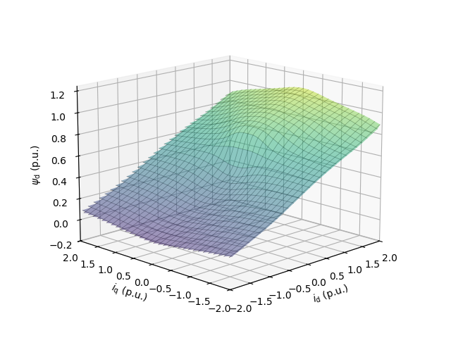
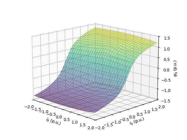
Load and plot the flux maps.

# Get the path of the MATLAB file and load the FEM data
p = Path(__file__).resolve().parent if "__file__" in globals() else Path.cwd()
fem_flux_map = utils.import_syre_data(str(p / "THOR.mat"))
utils.plot_map(fem_flux_map, "d", base, lims={"x": (-2, 2), "y": (-2, 2)})
utils.plot_map(fem_flux_map, "q", base, lims={"x": (-2, 2), "y": (-2, 2)})

Configure the system model.

# Create the machine model
fem_curr_map = fem_flux_map.invert()
par = model.SaturatedSynchronousMachinePars(n_p=2, R_s=0.2, i_s_dq_fcn=fem_curr_map)
machine = model.SynchronousMachine(par)
k = 0.1 * nom.tau / base.w_M**2  # Quadratic load torque profile
mechanics = model.MechanicalSystem(J=2 * 0.0042, B_L=lambda w_M: k * abs(w_M))
converter = model.VoltageSourceConverter(u_dc=310)
mdl = model.Drive(machine, mechanics, converter)

Configure the control system. Since the inertia estimate J is provided in CurrentVectorControllerCfg, the mechanical-model-based speed observer is used.

est_par = control.SaturatedSynchronousMachinePars(
    n_p=2, R_s=0.2, i_s_dq_fcn=fem_curr_map, psi_s_dq_fcn=fem_flux_map
)
cfg = control.CurrentVectorControllerCfg(i_s_max=2 * base.i, J=2 * 0.0042)
vector_ctrl = control.CurrentVectorController(est_par, cfg, sensorless=True)
speed_ctrl = control.SpeedController(J=2 * 0.0042, alpha_s=2 * pi * 4)
ctrl = control.VectorControlSystem(vector_ctrl, speed_ctrl)

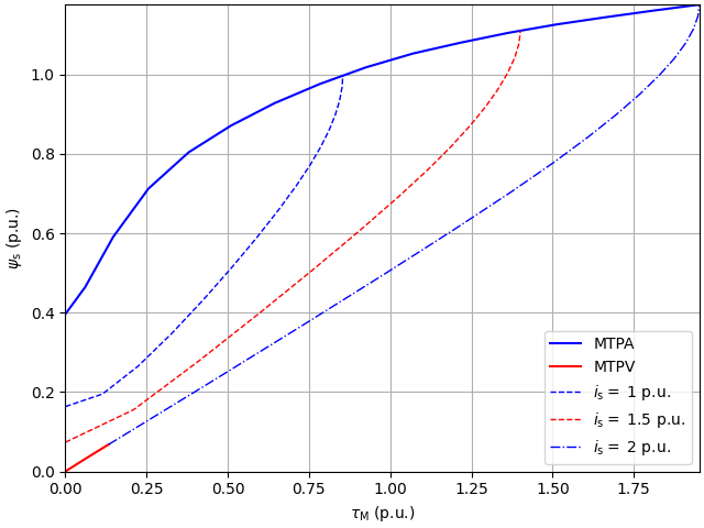
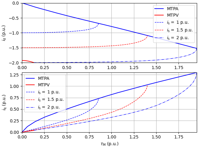
Plot control characteristics.

# sphinx_gallery_thumbnail_number = 4
i_s_vals = [1, 1.5, 2]  # Current values for the plots
mc = utils.MachineCharacteristics(est_par)
mc.plot_flux_vs_torque(i_s_vals, base)
mc.plot_current_vs_torque(i_s_vals, base)
mc.plot_current_loci(i_s_vals, base)
mc.plot_flux_loci(i_s_vals, base)

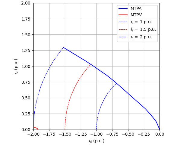
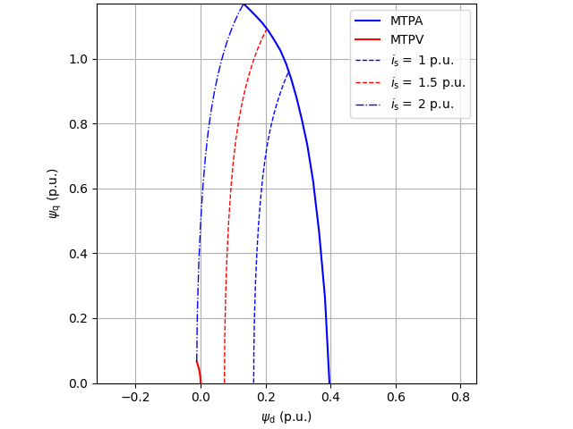
Set the speed reference and the external load torque.

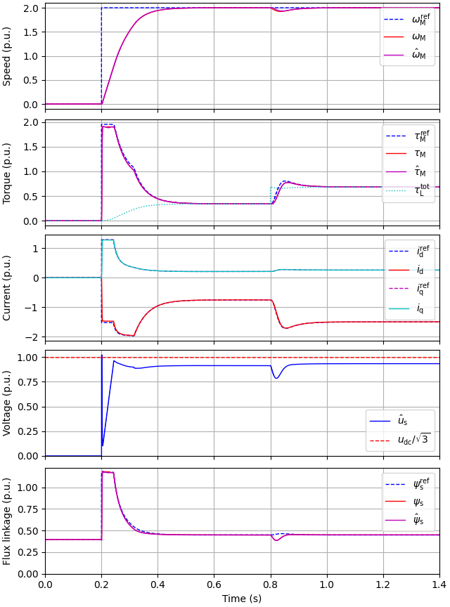
ctrl.set_speed_ref(lambda t: (t > 0.2) * 2 * base.w_M)
mdl.mechanics.set_external_load_torque(lambda t: (t > 0.8) * 0.4 * nom.tau)

Create the simulation object, simulate, and plot the results in per-unit values.

sim = model.Simulation(mdl, ctrl)
res = sim.simulate(t_stop=1.4)
utils.plot(res, base)

References

Total running time of the script: (0 minutes 37.630 seconds)

Gallery generated by Sphinx-Gallery