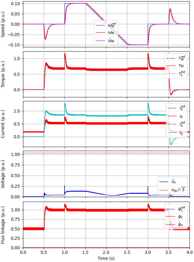
6.7-kW saturated SyRM, signal injection

This example simulates sensorless vector control of a saturated 6.7-kW synchronous reluctance machine (SyRM). Square-wave signal injection with a simple phase-locked loop is used. Cross-saturation errors are compensated for using flux maps. Square-wave signal injection with a simple phase-locked loop is used.

import matplotlib.pyplot as plt
import numpy as np

import motulator.drive.control.sm as control
from motulator.drive import model, utils

Compute base values based on the nominal values.

nom = utils.NominalValues(U=370, I=15.5, f=105.8, P=6.7e3, tau=20.1)
base = utils.BaseValues.from_nominal(nom, n_p=2)

Configure the system model.

# Use analytical saturation model
curr_map = utils.SaturationModelSyRM(
    a_d0=17.4, a_dd=373, S=5, a_q0=52.1, a_qq=658, T=1, a_dq=1120, U=1, V=0
)
par = model.SaturatedSynchronousMachinePars(
    n_p=2, R_s=0.54, i_s_dq_fcn=curr_map, kind="rel"
)
machine = model.SynchronousMachine(par)
mechanics = model.MechanicalSystem(J=0.015)
converter = model.VoltageSourceConverter(u_dc=540)
mdl = model.Drive(machine, mechanics, converter)

Configure the control system.

# Compute rectilinear current and flux maps
psi_d_range = np.linspace(-1.5 * base.psi, 1.5 * base.psi, 32)
psi_q_range = np.linspace(-0.5 * base.psi, 0.5 * base.psi, 32)
curr_map = curr_map.as_magnetic_model(psi_d_range, psi_q_range)
flux_map = curr_map.invert()

# Parameter estimates, stator resistance not needed
est_par = model.SaturatedSynchronousMachinePars(
    n_p=2, R_s=0, i_s_dq_fcn=curr_map, psi_s_dq_fcn=flux_map, kind="rel"
)
cfg = control.CurrentVectorControllerCfg(i_s_max=2 * base.i, psi_s_min=0.5 * base.psi)
vector_ctrl = control.SignalInjectionController(est_par, cfg)
speed_ctrl = control.SpeedController(J=0.015, alpha_s=2 * np.pi * 4)
ctrl = control.VectorControlSystem(vector_ctrl, speed_ctrl)

Set the speed reference and the external load torque.

t_stop = 4
times = np.array([0, 0.25, 0.25, 0.375, 0.5, 0.625, 0.75, 0.75, 1]) * t_stop
values = np.array([0, 0, 1, 1, 0, -1, -1, 0, 0]) * 0.1 * base.w_M
ctrl.set_speed_ref(utils.SequenceGenerator(times, values))

times = np.array([0, 0.125, 0.125, 0.875, 0.875, 1]) * t_stop
values = np.array([0, 0, 1, 1, 0, 0]) * nom.tau
mdl.mechanics.set_external_load_torque(utils.SequenceGenerator(times, values))

Create the simulation object, simulate, and plot the results in per-unit values.

sim = model.Simulation(mdl, ctrl)
res = sim.simulate(t_stop)
utils.plot(res, base)

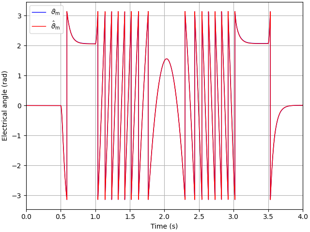
Plot also the angles.

plt.figure()
plt.plot(res.mdl.t, res.mdl.machine.theta_m, label=r"$\vartheta_\mathrm{m}$")
plt.plot(
    res.ctrl.t,
    res.ctrl.fbk.theta_m,
    ds="steps-post",
    label=r"$\hat \vartheta_\mathrm{m}$",
)
plt.legend()
plt.xlim(0, 4)
plt.xlabel("Time (s)")
plt.ylabel("Electrical angle (rad)")
plt.show()