5.1-kW saturated PM-SyRM, FVC

This example simulates sensorless flux-vector control (FVC) of a saturated 5.1-kW permanent-magnet synchronous reluctance machine (PM-SyRM). The flux maps of this example machine, known as THOR, are from the SyR-e project:

SyR-e/syre_public

The SyR-e project has been licensed under the Apache License, Version 2.0. We acknowledge the developers of the SyR-e project. The flux maps from other sources can be used in a similar manner.

The control system takes the saturation into account. This example also applies the mechanical-model-based speed observer.

from pathlib import Path

import numpy as np
from scipy.interpolate import LinearNDInterpolator

import motulator.drive.control.sm as control
from motulator.drive import model, utils

Compute base values based on the nominal values (just for figures).

nom = utils.NominalValues(U=220, I=15.6, f=85, P=5.07e3, tau=19)
base = utils.BaseValues.from_nominal(nom, n_p=2)

Load the flux maps.

# Get the path of the MATLAB file and load the FEM data
p = Path(__file__).resolve().parent if "__file__" in globals() else Path.cwd()
fem_flux_map = utils.import_syre_data(str(p / "THOR.mat"))

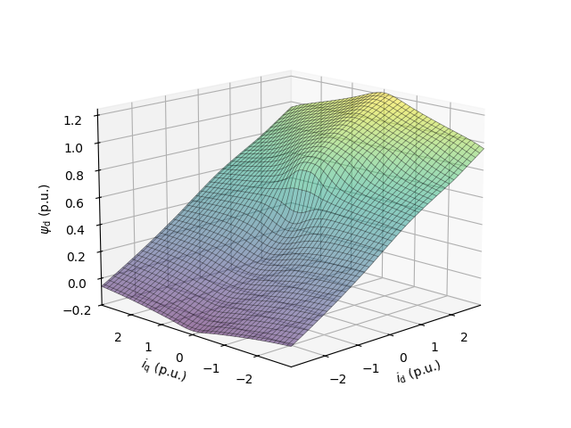
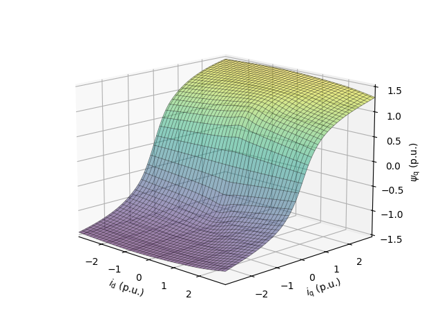
Plot the maps in per-unit values.

# sphinx_gallery_thumbnail_number = 3
utils.plot_map(fem_flux_map, "d", base, x_lims=(-2, 2), y_lims=(-2, 2))
utils.plot_map(fem_flux_map, "q", base, x_lims=(-2, 2), y_lims=(-2, 2))

• 
• 

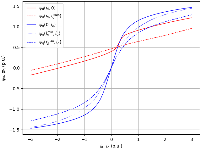
Two-dimensional presentation of flux maps.

utils.plot_flux_vs_current(fem_flux_map, base, lims=(-2, 2))

Configure the system model.

# Create the current map interpolator directly from the FEM data
points = np.column_stack(
    (np.real(fem_flux_map.psi_s_dq.ravel()), np.imag(fem_flux_map.psi_s_dq.ravel()))
)
mdl_curr_map = LinearNDInterpolator(points, fem_flux_map.i_s_dq.ravel())

# Machine model parameters
par = model.SaturatedSynchronousMachinePars(
    n_p=2,
    R_s=0.2,
    i_s_dq_fcn=lambda psi_s_dq: mdl_curr_map((np.real(psi_s_dq), np.imag(psi_s_dq))),
)
machine = model.SynchronousMachine(par)
k = 0.25 * nom.tau / base.w_M**2  # Quadratic load torque profile
mechanics = model.MechanicalSystem(J=2 * 0.0042, B_L=lambda w_M: k * abs(w_M))
converter = model.VoltageSourceConverter(u_dc=310)
mdl = model.Drive(machine, mechanics, converter)

Configure the control system.

# Create the flux and current maps for the control system
fem_curr_map = fem_flux_map.invert()
est_par = control.SaturatedSynchronousMachinePars(
    n_p=2, R_s=0.2, i_s_dq_fcn=fem_curr_map, psi_s_dq_fcn=fem_flux_map
)
# Since the inertia `J` is provided, the mechanical-model-based speed observer is used
cfg = control.FluxVectorControllerCfg(i_s_max=2 * base.i, J=2 * 0.0042, alpha_i=0)
vector_ctrl = control.FluxVectorController(est_par, cfg, sensorless=True)
speed_ctrl = control.SpeedController(J=2 * 0.0042, alpha_s=2 * np.pi * 4)
ctrl = control.VectorControlSystem(vector_ctrl, speed_ctrl)

Set the speed reference and the external load torque.

ctrl.set_speed_ref(lambda t: (t > 0.2) * 2 * base.w_M)

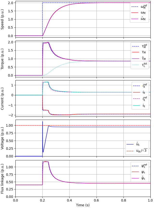
Create the simulation object, simulate, and plot the results in per-unit values.

sim = model.Simulation(mdl, ctrl)
res = sim.simulate(t_stop=1)
utils.plot(res, base)