5.6-kW saturated PM-SyRM, FVC#

This example simulates sensorless flux-vector control (FVC) of a 5.6-kW permanent-magnet synchronous reluctance machine (PM-SyRM, Baldor ECS101M0H7EF4) drive. The machine model is parametrized using the flux map data, measured using the constant-speed test.

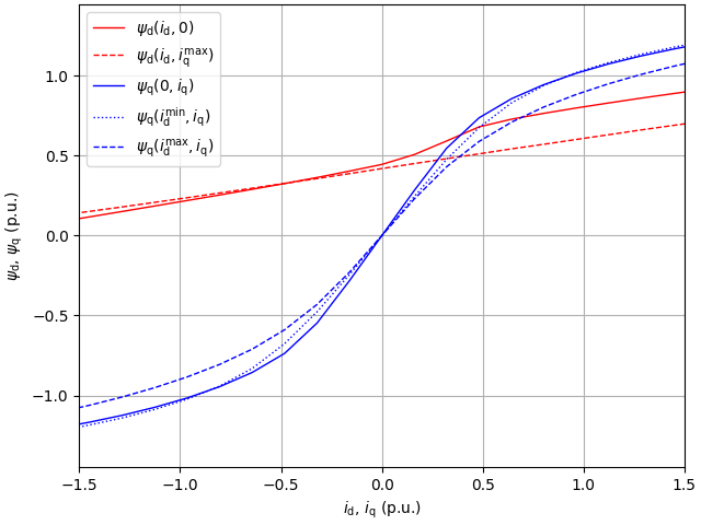
The control system is parametrized using an algebraic saturation model from [1], fitted to the measured data. For comparison, the measured data is plotted together with the model predictions.

This example also demonstrates the mechanical-model-based speed observer [2]. The lag of the speed estimate in accelerations is avoided, allowing to increase the speed-control bandwidth. Using the mechanical-model-based speed observer is particularly useful in the case of PM-SyRMs, where the speed-estimation bandwidth otherwise would be limited due to the comparatively large q-axis inductance.

from pathlib import Path

import numpy as np
from scipy.io import loadmat

import motulator.drive.control.sm as control
from motulator.drive import model, utils

Compute base values based on the nominal values (just for figures).

nom = utils.NominalValues(U=460, I=8.8, f=60, P=5.6e3, tau=29.7)
base = utils.BaseValues.from_nominal(nom, n_p=2)

Plot the saturation model (surfaces) and the measured flux map data (points). This data is used to parametrize the machine model.

# Load the measured data from the MATLAB file
p = Path(__file__).resolve().parent if "__file__" in globals() else Path.cwd()
meas_data = loadmat(p / "ABB_400rpm_map.mat")

# Create the flux map from the measured data
meas_flux_map = utils.MagneticModel(
    i_s_dq=meas_data["id_map"] + 1j * meas_data["iq_map"],
    psi_s_dq=meas_data["psid_map"] + 1j * meas_data["psiq_map"],
    type="flux_map",
)

# Plot the measured data
# sphinx_gallery_thumbnail_number = 4
utils.plot_flux_vs_current(meas_flux_map, base, x_lims=(-1.5, 1.5))

Create a saturation model, which will be used in the control system.

i_s_dq_fcn = utils.SaturationModelPMSyRM(
    a_d0=3.96,
    a_dd=28.5,
    S=4,
    a_q0=1.1 * 5.89,  # Unsaturated q-axis inductance is underestimated for robustness
    a_qq=2.67,
    T=6,
    a_dq=41.5,
    U=1,
    V=1,
    a_b=81.75,
    a_bp=1,
    k_q=0.1,
    psi_n=0.804,
    W=2,
)

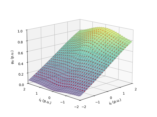
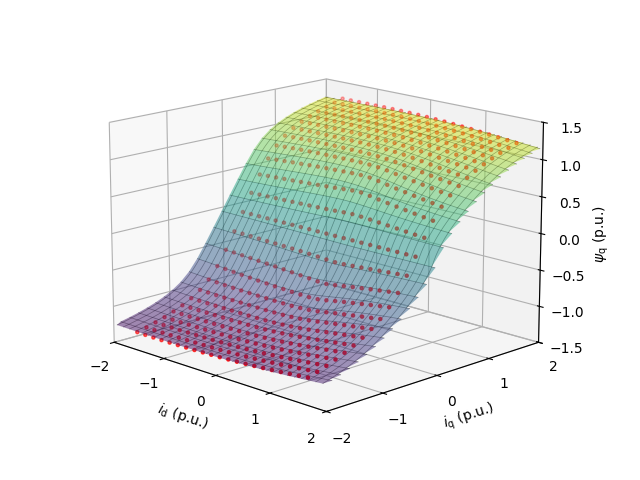
Compare the saturation model with the measured data.

# Generate the flux map using the saturation model
est_curr_map = i_s_dq_fcn.as_magnetic_model(
    d_range=np.linspace(-0.1 * base.psi, base.psi, 256),
    q_range=np.linspace(-1.4 * base.psi, 1.4 * base.psi, 256),
)
est_flux_map = est_curr_map.invert()

# Plot the saturation model (surface) and the measured data (points)
utils.plot_map(
    est_flux_map,
    "d",
    base,
    lims={"x": (-2, 2), "y": (-2, 2), "z": (0, 1)},
    ticks={"x": [-2, -1, 0, 1, 2], "y": [-2, -1, 0, 1, 2]},
    raw_data=meas_flux_map,
)
utils.plot_map(
    est_flux_map,
    "q",
    base,
    lims={"x": (-2, 2), "y": (-2, 2), "z": (-1.5, 1.5)},
    ticks={"x": [-2, -1, 0, 1, 2], "y": [-2, -1, 0, 1, 2]},
    raw_data=meas_flux_map,
)

Configure the system model.

meas_curr_map = meas_flux_map.invert()
par = model.SaturatedSynchronousMachinePars(n_p=2, R_s=0.63, i_s_dq_fcn=meas_curr_map)
machine = model.SynchronousMachine(par)
mechanics = model.MechanicalSystem(J=0.05)
converter = model.VoltageSourceConverter(u_dc=540)
mdl = model.Drive(machine, mechanics, converter)

Configure the control system. Since the inertia estimate J is provided in FluxVectorControllerCfg, the mechanical-model-based speed observer is used. Integral action in flux-vector control is not needed (alpha_i = 0) since the speed observer’s load-torque disturbance estimation provides integral action.

est_par = control.SaturatedSynchronousMachinePars(
    n_p=2, R_s=0.63, i_s_dq_fcn=est_curr_map, psi_s_dq_fcn=est_flux_map
)
cfg = control.FluxVectorControllerCfg(i_s_max=2 * base.i, J=0.05, alpha_i=0)
vector_ctrl = control.FluxVectorController(est_par, cfg, sensorless=True)
speed_ctrl = control.SpeedController(J=0.05, alpha_s=2 * np.pi * 4)
ctrl = control.VectorControlSystem(vector_ctrl, speed_ctrl)

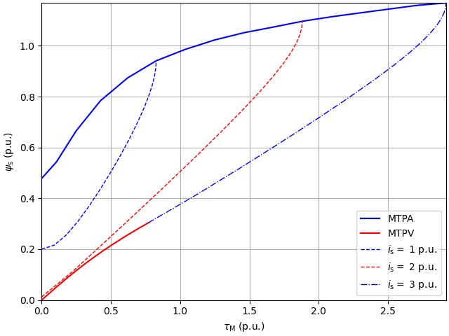
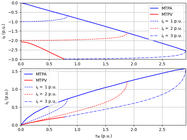
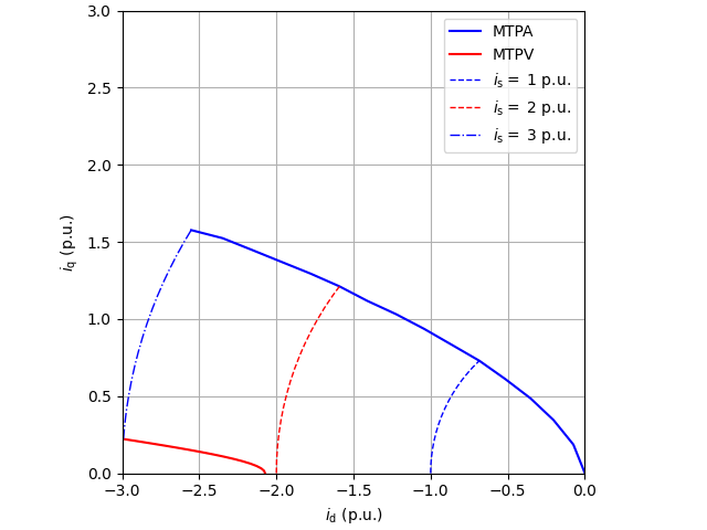
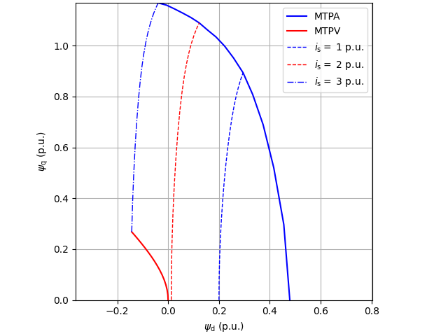
Visualize the control loci.

i_s_vals = [1, 2, 3]  # Current values for the plots
mc = utils.MachineCharacteristics(est_par)
mc.plot_flux_vs_torque(i_s_vals, base)
mc.plot_current_vs_torque(i_s_vals, base)
mc.plot_current_loci(i_s_vals, base)
mc.plot_flux_loci(i_s_vals, base)

Set the speed reference and the external load torque.

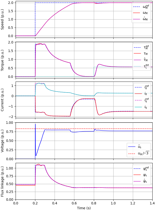
ctrl.set_speed_ref(lambda t: (t > 0.2) * 2 * base.w_M)
mdl.mechanics.set_external_load_torque(lambda t: (t > 0.8) * 0.7 * nom.tau)

Create the simulation object, simulate, and plot the results in per-unit values.

sim = model.Simulation(mdl, ctrl)
res = sim.simulate(t_stop=1.4)
utils.plot(res, base)

References

Total running time of the script: (0 minutes 26.020 seconds)

Gallery generated by Sphinx-Gallery