2.2-kW IM, LC filter, V/Hz control#

This example simulates open-loop V/Hz control of a 2.2-kW induction machine (IM) drive equipped with an output LC filter.

from math import inf, pi

import matplotlib.pyplot as plt

import motulator.drive.control.im as control
from motulator.drive import model, utils

Compute base values based on the nominal values (just for figures).

nom = utils.NominalValues(U=400, I=5, f=50, P=2.2e3, tau=14.6)
base = utils.BaseValues.from_nominal(nom, n_p=2)

Create the system model, filter parameters correspond to [1].

par = model.InductionMachineInvGammaPars(
    n_p=2, R_s=3.7, R_R=2.1, L_sgm=0.021, L_M=0.224
)
machine = model.InductionMachine(par)
k = 1.1 * nom.tau / base.w_M**2  # Quadratic load torque profile
mechanics = model.MechanicalSystem(J=0.015, B_L=lambda w_M: k * abs(w_M))
converter = model.VoltageSourceConverter(u_dc=540)
lc_filter = model.LCFilter(L_f=8e-3, C_f=9.9e-6, R_f=0.1)
mdl = model.Drive(machine, mechanics, converter, lc_filter, pwm=True)

Control system (parametrized as open-loop V/Hz control).

est_par = control.InductionMachineInvGammaPars(n_p=2, R_s=0, R_R=0, L_sgm=0, L_M=inf)
cfg = control.ObserverBasedVHzControllerCfg(
    psi_s_nom=base.psi, i_s_max=inf, alpha_f=0, alpha_tau=0, alpha_psi=0
)
vhz_ctrl = control.ObserverBasedVHzController(est_par, cfg)
ctrl = control.VHzControlSystem(vhz_ctrl, slew_rate=2 * pi * 60)

Set the speed reference. The external load torque is zero by default.

ctrl.set_speed_ref(lambda t: (t > 0.2) * base.w_M)

Create the simulation object, simulate, and plot the results in per-unit values.

sim = model.Simulation(mdl, ctrl)
res = sim.simulate(t_stop=1.4)
# sphinx_gallery_thumbnail_number = 2
utils.plot(res, base)

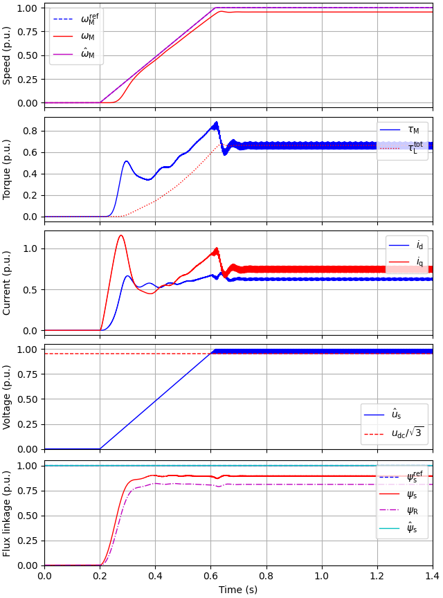
Plot additional waveforms.

t_lims = (1.1, 1.125)  # Time span for the zoomed-in plot

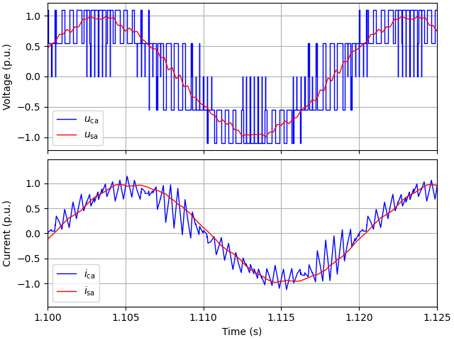
# Plot the converter and stator voltages (phase a)
fig1, (ax1, ax2) = plt.subplots(2, 1)
ax1.plot(res.mdl.t, res.mdl.converter.u_c_ab.real / base.u, label=r"$u_\mathrm{ca}$")
ax1.plot(res.mdl.t, res.mdl.machine.u_s_ab.real / base.u, label=r"$u_\mathrm{sa}$")
ax1.set_xlim(t_lims)
ax1.legend()
ax1.set_xticklabels([])
ax1.set_ylabel("Voltage (p.u.)")
# Plot the converter and stator currents (phase a)
ax2.plot(res.mdl.t, res.mdl.converter.i_c_ab.real / base.i, label=r"$i_\mathrm{ca}$")
ax2.plot(res.mdl.t, res.mdl.machine.i_s_ab.real / base.i, label=r"$i_\mathrm{sa}$")
ax2.set_xlim(t_lims)
ax2.legend()
ax2.set_ylabel("Current (p.u.)")
ax2.set_xlabel("Time (s)")

plt.show()

References

Total running time of the script: (0 minutes 7.385 seconds)

Gallery generated by Sphinx-Gallery