28-kW PM-SyRM, train flux map, measured data

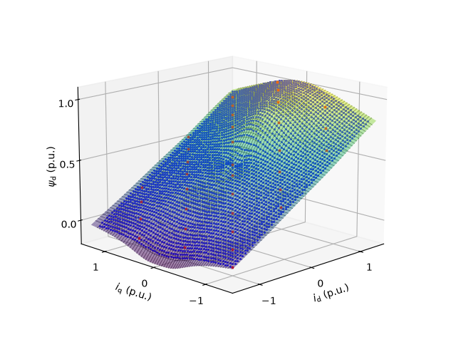
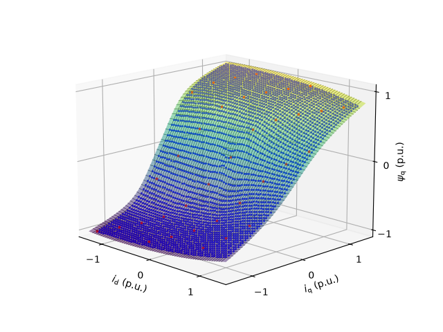
This example trains a GradNet flux-linkage map for a 10-pole 28-kW PM synchronous reluctance machine (Brusa HSM1.10.18.04) from a measured dataset.

from pathlib import Path

import numpy as np

import motulator.drive.gradnet as gn
from motulator.drive import utils

Get nominal and base values, needed for figures only.

nom = utils.NominalValues(U=283, I=78, f=408, P=25e3, tau=49)
base = utils.BaseValues.from_nominal(nom, n_p=5)

Set up the paths and parameters.

p = Path(__file__).resolve().parent if "__file__" in globals() else Path.cwd()

dataset_path = p / "datasets/brusa_meas.npz"
trained_path = p / "trained_models/brusa_meas_flux_map_pnorm_d12_sub100.pth"
subsample = 100
activation = gn.PNormGradient

Train the model.

if not trained_path.exists():
    gn.train_gradnet(
        dataset_path=dataset_path,
        base=base,
        save_model_path=trained_path,
        is_flux_map=True,
        embed_dim=12,
        epochs=20000,
        subsample=subsample,
        activation=activation,
    )

Create the GradNet model and its callable.

model = gn.load_gradnet(trained_path, activation=activation)
flux_map_fcn = gn.FluxMap(model)

Load the dataset for comparison and split it into training and validation sets.

train_data, val_data = gn.get_training_data(
    str(dataset_path), base=base, subsample=subsample
)

Plot the flux map.

# Sample the map on a grid for plotting
flux_map = gn.sample_map_on_grid(
    flux_map_fcn,
    map_type="flux_map",
    d_range=np.linspace(-1.4, 1.4, 50) * base.i,
    q_range=np.linspace(-1.4, 1.4, 50) * base.i,
)

# Constant current contours corresponding to the measured dataset, for visualization
i_d_levels = np.arange(-145, 146, 5) / base.i
i_q_levels = np.arange(-145, 145, 5) / base.i
current_loci_levels = (i_d_levels, i_q_levels)

gn.plot_maps(
    flux_map,
    "d",
    base,
    current_loci=True,
    lims={"x": (-1.5, 1.5), "y": (-1.5, 1.5), "z": (-0.2, 1.1)},
    ticks={"x": [-1, 0, 1], "y": [-1, 0, 1], "z": [0, 0.5, 1]},
    raw_data=[val_data, train_data],
    current_loci_levels=current_loci_levels,
)

gn.plot_maps(
    flux_map,
    "q",
    base,
    current_loci=True,
    lims={"x": (-1.5, 1.5), "y": (-1.5, 1.5), "z": (-1.1, 1.1)},
    ticks={"x": [-1, 0, 1], "y": [-1, 0, 1], "z": [-1, 0, 1]},
    raw_data=[val_data, train_data],
    current_loci_levels=current_loci_levels,
)

• 
• 

Print error metrics.

gn.print_flux_map_errors_meas(flux_map_fcn, val_data, base=base)

Flux-map error metrics: rmse=0.011 p.u., max=0.075 p.u., std=0.007 p.u.