5.6-kW PM-SyRM, GradNet from measured data, FVC

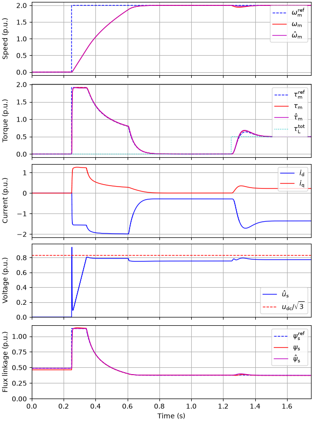
This example simulates flux-vector control (FVC) of a 5.6-kW PM synchronous reluctance machine (Baldor ECS101M0H7EF4) drive. GradNet models trained on measured data without spatial harmonics are used for both the machine model and the control system.

from pathlib import Path

import numpy as np

import motulator.drive.control.sm as control
import motulator.drive.gradnet as gn
from motulator.drive import model, utils

Compute base values based on the nominal values (just for figures).

nom = utils.NominalValues(U=460, I=8.8, f=60, P=5.6e3, tau=29.7)
base = utils.BaseValues.from_nominal(nom, n_p=2)

Determine the path of the current script.

p = Path(__file__).resolve().parent if "__file__" in globals() else Path.cwd()

Configure the system model using the GradNet current map, without spatial harmonics, trained on the measured dataset.

path = "trained_models/baldor_meas_curr_map_squareplus_d12_sub10.pth"
gradnet = gn.load_gradnet(p / path, activation=gn.Squareplus)
current_map = gn.CurrentMap(gradnet)
par = model.SaturatedSynchronousMachinePars(n_p=2, R_s=0.63, i_s_dq_fcn=current_map)

machine = model.SynchronousMachine(par)
mechanics = model.MechanicalSystem(J=0.05)
converter = model.VoltageSourceConverter(u_dc=540)
mdl = model.Drive(machine, mechanics, converter)

Configure the control system using the GradNet flux map, without spatial harmonics, trained on the measured dataset.

# Parametrize the estimated machine model
path = "trained_models/baldor_meas_flux_map_pnorm_d6_sub10.pth"
est_flux_map = gn.FluxMap(gn.load_gradnet(p / path, activation=gn.PNormGradient))
est_par = control.SaturatedSynchronousMachinePars(
    n_p=2, R_s=0.63, psi_s_dq_fcn=est_flux_map
)

# Configure the control system
cfg = control.FluxVectorControllerCfg(
    i_s_max=2 * base.i, alpha_i=0, alpha_o=2 * np.pi * 8, J=0.05, sensorless=False
)
vector_ctrl = control.FluxVectorController(est_par, cfg)
speed_ctrl = control.SpeedController(J=0.05, alpha_s=2 * np.pi * 4)
ctrl = control.VectorControlSystem(vector_ctrl, speed_ctrl)

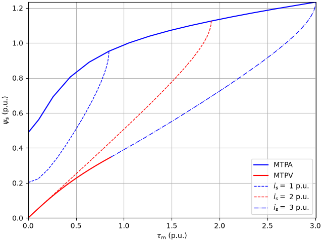
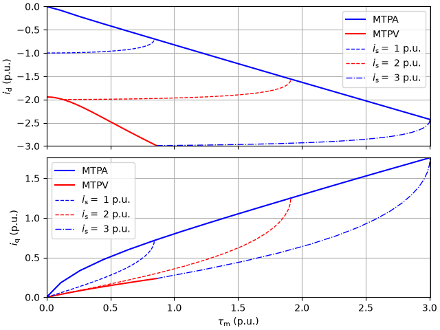
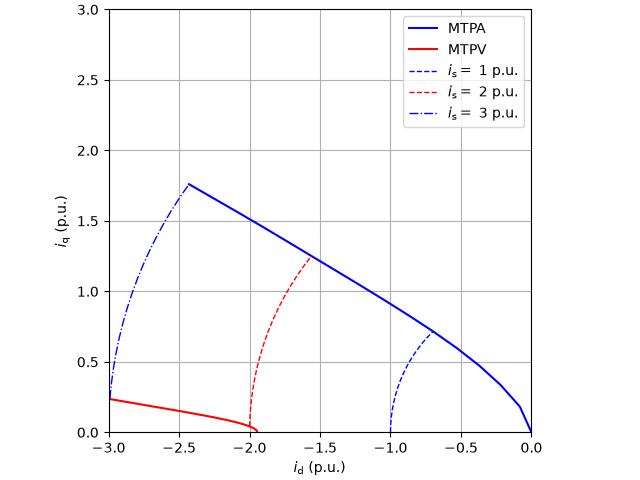
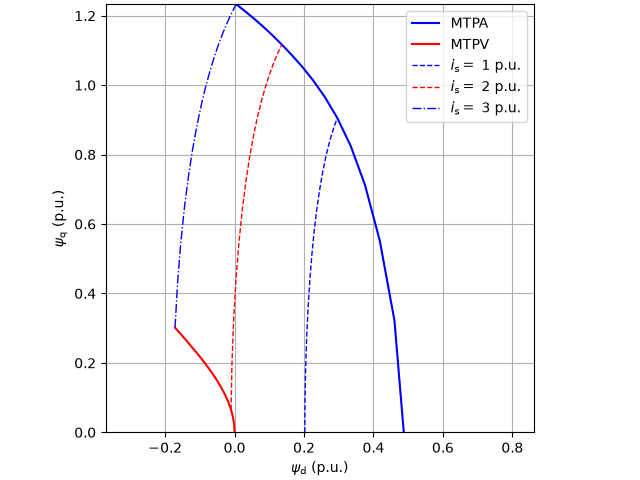
Visualize the control loci.

i_s_vals = [1, 2, 3]  # Current values for the plots
mc = utils.MachineCharacteristics(est_par)
mc.plot_flux_vs_torque(i_s_vals, base)
mc.plot_current_vs_torque(i_s_vals, base)
mc.plot_current_loci(i_s_vals, base)
mc.plot_flux_loci(i_s_vals, base)

• 
• 
• 
• 

Set the speed reference and the external load torque.

ctrl.set_speed_ref(lambda t: (t > 0.25) * 2 * base.w_M)
mdl.mechanics.set_external_load_torque(lambda t: (t > 1.25) * 0.5 * base.tau)

Create the simulation object, simulate, and plot the results in per-unit values.

sim = model.Simulation(mdl, ctrl)
res = sim.simulate(t_stop=1.75)
utils.plot(res, base)