5.6-kW PM-SyRM, train flux map, FEM data with spatial harmonics

This example trains a GradNet flux-linkage map for a four-pole 5.6-kW PM synchronous reluctance machine (ABB Baldor ECS101M0H7EF4) from a FEM dataset with spatial harmonics.

from pathlib import Path

import numpy as np

import motulator.drive.gradnet as gn
from motulator.drive import utils

Set nominal and base values.

nom = utils.NominalValues(U=460, I=8.8, f=60, P=5.6e3, tau=29.7)
base = utils.BaseValues.from_nominal(nom, n_p=2)

Set up the paths and parameters.

p = Path(__file__).resolve().parent if "__file__" in globals() else Path.cwd()

Flux map with spatial harmonics, trained on FEM data.

dataset_path = p / "datasets/baldor_fem.npz"
trained_path = p / "trained_models/baldor_fem_flux_map_harm_pnorm_d48_sub10.pth"
subsample = 10
k = 6
activation = gn.PNormGradient

Train the model.

if not trained_path.exists():
    gn.train_gradnet(
        dataset_path=dataset_path,
        base=base,
        save_model_path=trained_path,
        is_flux_map=True,
        k=k,
        embed_dim=48,
        epochs=1000,
        subsample=subsample,
        activation=activation,
    )

Load the dataset for visualization comparison.

# Get the training and validation data (complement) from the helper function
# Note: get_training_data returns (psi, i, ...), but we need (i, psi, ...)
(trn_psi, trn_i, trn_theta, trn_tau), (val_psi, val_i, val_theta, val_tau) = (
    gn.get_training_data(
        str(dataset_path),
        base=base,
        subsample=subsample,
        other_keys=["theta_m", "tau_m"],
    )
)
trn_data = (trn_i, trn_psi, trn_theta, trn_tau)
val_data = (val_i, val_psi, val_theta, val_tau)

Load the GradNet model and create its callable.

model = gn.load_gradnet(trained_path, activation=activation)
harm_map = gn.FluxMapWithHarmonics(model, k=k)

Evaluate the model at single point.

i_s_dq_mtpa = -9 + 9j  # Approximately the rated MTPA current
theta_m = np.deg2rad(30)
psi_s_dq, tau_m = harm_map(i_s_dq_mtpa, np.exp(1j * theta_m))
print(f"Current: {i_s_dq_mtpa:.2f} A")
print(f"Angle: {np.rad2deg(theta_m):.2f} deg")
print(f"Flux linkage: {psi_s_dq:.2f} Vs")
print(f"Torque per pole pair: {tau_m:.2f} Nm")

Current: -9.00+9.00j A
Angle: 30.00 deg
Flux linkage: 0.29+0.82j Vs
Torque per pole pair: 13.69 Nm

Plot torque surface.

# Define ranges for visualization
i_q_range = np.linspace(0, 2 * base.i, 50)
theta_m_range = np.linspace(0, 2 * np.pi / k, 50)

# Plot torque as a function of i_q and theta_m at fixed i_d
gn.plot_surface_vs_current_and_angle(
    current_range=i_q_range,
    fixed_value=i_s_dq_mtpa.real,
    theta_m_range=theta_m_range,
    map_fcn=harm_map,
    input="i_q",
    output="tau_m",
    val_data=val_data,
    trn_data=trn_data,
    opts=gn.PlotOptions(
        base=base,
        lims={"x": (0, 2), "y": (0, 60), "z": (0, 1.5)},
        ticks={"x": [0, 1, 2], "y": [0, 30, 60], "z": [0, 0.5, 1.0, 1.5]},
        loci_levels_source="val",
    ),
)

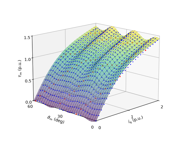
Plot torque vs angle.

theta_m_range = np.linspace(0, 2 * np.pi / k, 120)
gn.plot_output_vs_angle(
    fixed_value=i_s_dq_mtpa,
    theta_m_range=theta_m_range,
    map_fcn=harm_map,
    val_data=val_data,
    trn_data=trn_data,
    opts=gn.PlotOptions(
        base=base,
        lims={"x": (0, 60), "y": (0, 1)},
        ticks={"x": [0, 15, 30, 45, 60], "y": [0, 0.2, 0.4, 0.6, 0.8, 1.0]},
    ),
)

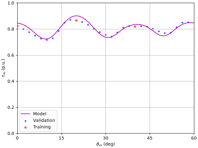
Print statistical error metrics on validation data.

val_dict = {
    "i_s_dq": val_i,
    "psi_s_dq": val_psi,
    "theta_m": val_theta,
    "tau_m": val_tau,
}
gn.print_flux_map_errors_fem(map_fcn=harm_map, raw_data=val_dict, base=base)

Error metrics:
Flux linkage: rmse=0.018 p.u., max=0.071 p.u., std=0.009 p.u.
Torque: rmse=0.016 p.u., max=0.115 p.u., std=0.011 p.u.