2.2-kW IM, dead time, CVC#

This example simulates sensorless current-vector control (CVC) of a 2.2-kW induction motor (IM) drive at low speeds. The dead time of the converter is modeled, and its effect is compensated for in the control system. The magnetic saturation is included in the machine model and taken into account in the control system. The sensorless observer and the compensation method are similar to [1].

from math import pi

import numpy as np

import motulator.drive.control.im as control
from motulator.common.utils import dead_time_error
from motulator.drive import model, utils

Compute base values based on the nominal values (just for figures).

nom = utils.NominalValues(U=400, I=5, f=50, P=2.2e3, tau=14.6)
base = utils.BaseValues.from_nominal(nom, n_p=2)

Away from the duty-ratio limits, the duty-ratio error caused by the dead time t_d is t_d/(2*T_s)*sign(i) in each phase, where i is the phase current and T_s is the half carrier period, equal to the sampling period. As in [1], the signum function is replaced with a smooth arctangent function, which approximates the effect of the parasitic capacitances of the power devices at low currents.

t_d = 2e-6  # Dead time (s)
T_s = 125e-6  # Sampling period (s), the default value in CurrentVectorControllerCfg


def smooth_sign(i):
    """Smooth approximation of the signum function."""
    return 2 / pi * np.arctan(i / (0.03 * base.i))

Configure the system model. The Γ-equivalent machine model with main-flux saturation is used. The parameters are based on the measured data of a 2.2-kW machine [2]. The dead time is a parameter of the converter.

par = model.InductionMachinePars(
    n_p=2, R_s=3.7, R_r=2.5, L_ell=0.023, L_s=lambda psi: 0.34 / (1 + (0.84 * psi) ** 7)
)


def create_model():
    machine = model.InductionMachine(par)
    mechanics = model.MechanicalSystem(J=0.015)
    converter = model.VoltageSourceConverter(u_dc=540, t_d=t_d, sign=smooth_sign)
    mdl = model.Drive(machine, mechanics, converter)
    mdl.mechanics.set_external_load_torque(lambda t: (t > 0.8) * 0.7 * nom.tau)
    return mdl

Configure the control system. If the duty-ratio error is given, the PWM compensates for it, and the realized voltage fed to the observer includes it. The speed reference is reversed under the load torque, leading to the regenerating mode.

def create_control_system(pwm=None):
    est_par = par  # Assume the machine model is perfectly known
    cfg = control.CurrentVectorControllerCfg(
        psi_s_nom=0.95 * base.psi, i_s_max=1.5 * base.i, sensorless=True
    )
    vector_ctrl = control.CurrentVectorController(est_par, cfg)
    speed_ctrl = control.SpeedController(J=0.015, alpha_s=2 * pi * 4)
    ctrl = control.VectorControlSystem(vector_ctrl, speed_ctrl, pwm)
    ctrl.set_speed_ref(lambda t: ((t > 0.2) - 2 * (t > 1.4)) * 0.05 * base.w_M)
    return ctrl

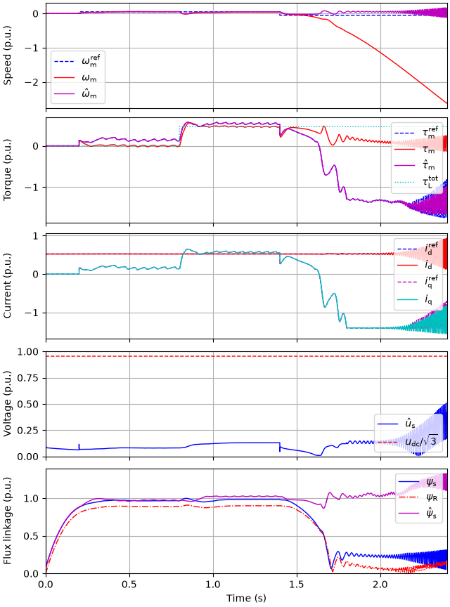
Simulate without the compensation. The voltage error caused by the dead time corrupts the flux and speed estimates. After the speed reversal, the drive fails in the regenerating mode.

sim = model.Simulation(create_model(), create_control_system())
res = sim.simulate(t_stop=2.4)
utils.plot(res, base)

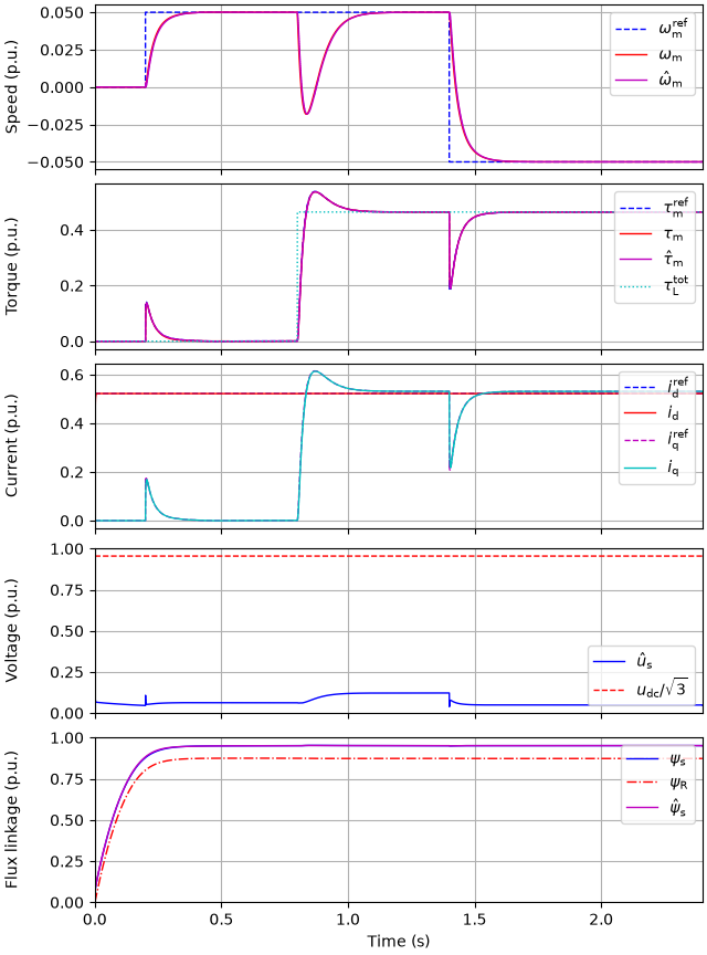
Simulate with the compensation, using the same duty-ratio error model as in the system model.

pwm = control.PWM(d_err=lambda i, d: dead_time_error(i, d, t_d, T_s, sign=smooth_sign))
sim = model.Simulation(create_model(), create_control_system(pwm))
res = sim.simulate(t_stop=2.4)
utils.plot(res, base)

# sphinx_gallery_thumbnail_number = 2

References

Total running time of the script: (0 minutes 21.239 seconds)

Gallery generated by Sphinx-Gallery