2.2-kW IPMSM, DPWM, FVC

This example compares space-vector PWM (SVPWM) and discontinuous PWM (DPWM) [1] in flux-vector control (FVC) of a 2.2-kW interior permanent-magnet synchronous machine (IPMSM) drive. The converter is modeled by carrier comparison, so the switching ripple of the currents is included. The drive operates at the nominal torque and a constant speed.

from math import pi

import matplotlib.pyplot as plt
import numpy as np

import motulator.drive.control.sm as control
from motulator.common.utils import complex2abc, set_style
from motulator.drive import model, utils

Compute base values based on the nominal values.

nom = utils.NominalValues(U=370, I=4.3, f=75, P=2.2e3, tau=14)
base = utils.BaseValues.from_nominal(nom, n_p=3)

Configure the machine model. The parameters are assumed to be accurately known in the control system.

par = model.SynchronousMachinePars(n_p=3, R_s=3.6, L_d=0.036, L_q=0.051, psi_f=0.545)

In the linear modulation range, DPWM clamps each leg to a DC rail for 120° of the fundamental period, so its average switching frequency is about 2/3 of the carrier frequency. DPWM1 clamps the legs in the segments centered at the peaks of the phase voltage and DPWM2 in the segments following the peaks, which suit the current lagging the voltage in the motoring mode. The methods are compared at the same nominal average switching frequency of 2 kHz: the sampling period of SVPWM is 250 µs, and that of DPWM is 2/3 of it. The duty ratios are updated twice per carrier period, i.e., the carrier frequency is 2 kHz in SVPWM and 3 kHz in DPWM. The rotor speed is constant, and the measured rotor angle is used, so that the results depend only on the modulation.

METHODS = ["SVPWM", "DPWM1", "DPWM2"]


def simulate(method, w_M, t_stop):
    """Simulate the drive at the nominal torque and the constant speed `w_M`."""
    mdl = model.Drive(
        model.SynchronousMachine(par),
        model.ExternalRotorSpeed(),
        model.VoltageSourceConverter(u_dc=540, modulator=model.CarrierComparison()),
        sensors=model.DriveSensors(theta_M=model.Sensor()),  # Sensored control
    )
    mdl.mechanics.set_external_rotor_speed(w_M)
    T_s = 250e-6 if method == "SVPWM" else 2 / 3 * 250e-6
    cfg = control.FluxVectorControllerCfg(
        i_s_max=1.5 * base.i, sensorless=False, T_s=T_s
    )
    vector_ctrl = control.FluxVectorController(par, cfg)
    ctrl = control.VectorControlSystem(vector_ctrl, pwm=control.PWM(method=method))
    ctrl.set_torque_ref(nom.tau)
    return model.Simulation(mdl, ctrl).simulate(t_stop=t_stop, N_eval=10)

The results are evaluated over an integer number of fundamental periods in the steady state. The switching instants are obtained by replaying the duty ratios through the carrier comparison, and the switching losses are approximated to be proportional to the switched current. The current ripple is the RMS value of the phase currents after removing the fundamental component, which is constant in rotor coordinates.

def evaluate(res, t_start, t_end):
    """Compute the operating point, switching, and current ripple."""
    ctrl, mdl = res.ctrl, res.mdl
    # Changes of the gate states and their instants
    carrier = model.CarrierComparison()
    t_sw, dq_abc, q_old = [], [], np.zeros(3)
    for t_k, T_s, d_abc in zip(ctrl.t, ctrl.ref.T_s, ctrl.ref.d_abc, strict=True):
        t_steps, gates = carrier(T_s, d_abc)
        for t, q in zip(t_k + np.cumsum(t_steps) - t_steps, gates[:, 0], strict=True):
            if t_start <= t < t_end:
                t_sw.append(t)
                dq_abc.append(np.abs(q - q_old))
            q_old = q
    dq_abc = np.array(dq_abc)
    i_abc = complex2abc(np.interp(t_sw, mdl.t, mdl.machine.i_s_ab)).T
    # Each sample is weighted by the time to the next one (exact for the voltage)
    m = (mdl.t >= t_start) & (mdl.t <= t_end)
    t = mdl.t[m]
    exp_j_theta_m = np.exp(1j * par.n_p * mdl.mechanics.theta_M[m])

    def mean(x):
        return np.sum(x[:-1] * np.diff(t)) / (t[-1] - t[0])

    u_s_dq = mean(mdl.machine.u_s_ab[m] / exp_j_theta_m)
    i_s_dq = mean(mdl.machine.i_s_ab[m] / exp_j_theta_m)
    di_s_ab = mdl.machine.i_s_ab[m] - i_s_dq * exp_j_theta_m
    return {
        "m": abs(u_s_dq) / (540 / np.sqrt(3)),  # Modulation index
        "phi": np.degrees(np.angle(u_s_dq / i_s_dq)),  # Power-factor angle
        "f_sw": np.sum(dq_abc) / 3 / 2 / (t_end - t_start),
        "p_sw": np.sum(dq_abc * np.abs(i_abc)) / (t_end - t_start),
        "ripple": np.sqrt(mean(np.abs(di_s_ab) ** 2) / 2) / base.i,
    }

Simulate the methods at a low and a high modulation index, i.e., the ratio of the fundamental voltage to its maximum u_dc/sqrt(3) in the linear modulation range. Print the realized switching frequency, the switching losses relative to SVPWM, and the current ripple. At the boundaries of the clamped segments, a leg may switch at the start of a half carrier period, so the realized switching frequency of DPWM is slightly higher than the nominal one.

T_SETTLE = 0.05
results = {}
for w_pu, n_periods in [(0.3, 1), (1.0, 3)]:
    T_1 = 2 * pi / (par.n_p * w_pu * base.w_M)  # Fundamental period
    t_end = T_SETTLE + n_periods * T_1
    for method in METHODS:
        res = simulate(method, w_pu * base.w_M, t_end + 1e-3)
        results[w_pu, method] = res, evaluate(res, T_SETTLE, t_end)
    ref = results[w_pu, "SVPWM"][1]
    print(
        f"Speed {w_pu} p.u.: modulation index {ref['m']:.2f}, "
        f"current lags by {ref['phi']:.0f}°"
    )
    for method in METHODS:
        ind = results[w_pu, method][1]
        f_sw, p_sw, ripple = ind["f_sw"] / 1e3, ind["p_sw"] / ref["p_sw"], ind["ripple"]
        print(
            f"  {method}: {f_sw:.2f} kHz, losses {p_sw:.2f}, ripple {ripple:.4f} p.u."
        )

Speed 0.3 p.u.: modulation index 0.33, current lags by 16°
  SVPWM: 2.00 kHz, losses 1.00, ripple 0.0138 p.u.
  DPWM1: 2.02 kHz, losses 0.79, ripple 0.0174 p.u.
  DPWM2: 2.03 kHz, losses 0.79, ripple 0.0169 p.u.
Speed 1.0 p.u.: modulation index 0.95, current lags by 19°
  SVPWM: 2.00 kHz, losses 1.00, ripple 0.0274 p.u.
  DPWM1: 2.08 kHz, losses 0.84, ripple 0.0199 p.u.
  DPWM2: 2.08 kHz, losses 0.82, ripple 0.0184 p.u.

Plot the duty ratio and the current of phase a over one fundamental period at the nominal speed. Since the current lags the voltage, the clamped segments of DPWM2 are closer to the current peaks than those of DPWM1. In DPWM2, the duty ratio of phase a approaches zero at the end of the segment in which phase c is clamped to the negative rail, where the voltages of the phases a and c are equal.

set_style()
_, axes = plt.subplots(2, len(METHODS), figsize=(10, 5), sharex=True, sharey="row")
T_1 = 2 * pi / (par.n_p * base.w_M)
for col, method in enumerate(METHODS):
    res = results[1.0, method][0]
    ax1, ax2 = axes[0, col], axes[1, col]
    ax1.plot(1e3 * (res.ctrl.t - T_SETTLE), res.ctrl.ref.d_abc[:, 0], ds="steps-post")
    i_a = complex2abc(res.mdl.machine.i_s_ab)[0]
    ax2.plot(1e3 * (res.mdl.t - T_SETTLE), i_a / base.i)
    ax1.set_title(method)
    ax2.set_xlabel("Time (ms)")
axes[0, 0].set_xlim(0, 1e3 * T_1)
axes[0, 0].set_ylabel(r"$d_\mathrm{a}$")
axes[1, 0].set_ylabel(r"$i_\mathrm{a}$ (p.u.)")
for ax in axes[:, 1:].flat:
    ax.tick_params(labelleft=True)
plt.show()

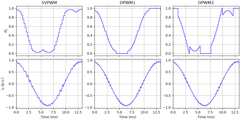
At the same nominal average switching frequency, DPWM gives a lower current ripple than SVPWM only at the high modulation index. DPWM1 and DPWM2 reduce the switching losses by 15–20 %. At the nominal speed, DPWM2 reduces them slightly more, since its clamped segments are closer to the current peaks.

References

[1]

Hava, Kerkman, Lipo, “A high-performance generalized discontinuous PWM algorithm,” IEEE Trans. Ind. Appl., 1998, https://doi.org/10.1109/28.720446