Note
Go to the end to download the full example code.
5.6-kW saturated PM-SyRM, discrete-time current control#
This example compares the continuous-time and direct discrete-time designs of the current controller [1] in sensorless current-vector control of a saturated 5.6-kW permanent-magnet synchronous reluctance machine (PM-SyRM). The sampling frequency is 5 kHz and the current-control bandwidth is 2π·500 rad/s, which is high compared with the sampling frequency.
Compute base values based on the nominal values.
nom = utils.NominalValues(U=460, I=8.8, f=60, P=5.6e3, tau=29.7)
base = utils.BaseValues.from_nominal(nom, n_p=2)
Configure the machine parameters based on the measured flux map, see 5.6-kW saturated PM-SyRM, FVC.
p = Path(utils.__file__).resolve().parents[3] / "examples/drive/data"
data = np.load(p / "baldor_400rpm_map.npz")
flux_map = utils.MagneticModel(
    i_s_dq=data["i_s_dq"], psi_s_dq=data["psi_s_dq"], type="flux_map"
)
par = model.SaturatedSynchronousMachinePars(
    n_p=2, R_s=0.63, i_s_dq_fcn=flux_map.invert()
)
The control system uses an analytical saturation model fitted to the measured data, so the model has small errors.
est_current_map = utils.SaturationModelPMSyRM(
    a_d0=3.96,
    a_dd=28.5,
    S=4,
    a_q0=5.89,
    a_qq=2.67,
    T=6,
    a_dq=41.5,
    U=1,
    V=1,
    a_b=81.75,
    a_bp=1,
    k_q=0.1,
    psi_n=0.804,
    W=2,
).as_magnetic_model(
    d_range=np.linspace(-0.1 * base.psi, base.psi, 256),
    q_range=np.linspace(-1.4 * base.psi, 1.4 * base.psi, 256),
)
est_par = control.SaturatedSynchronousMachinePars(
    n_p=2, R_s=0.63, psi_s_dq_fcn=est_current_map.invert()
)
Simulate the drive in torque-control mode at the constant speed of 1.5 p.u. The discrete-time design compensates for the delays itself, which is taken into account in the PWM configuration.
def simulate(discrete: bool):
    mdl = model.Drive(
        model.SynchronousMachine(par),
        model.ExternalRotorSpeed(),
        model.VoltageSourceConverter(u_dc=540),
        pwm=True,
    )
    mdl.mechanics.set_external_rotor_speed(lambda t: 1.5 * base.w_M)
    cfg = control.CurrentVectorControllerCfg(
        i_s_max=2 * base.i,
        alpha_c=2 * pi * 500,
        alpha_ref=2 * pi * 500,  # Fast reference generation
        online_ref=True,
        T_s=200e-6,
        discrete=discrete,
    )
    pwm = control.PWM(k_comp=0) if discrete else None
    vector_ctrl = control.CurrentVectorController(est_par, cfg)
    vector_ctrl.observer.speed_observer.w_M = 1.5 * base.w_M  # Initial speed estimate
    ctrl = control.VectorControlSystem(vector_ctrl, pwm=pwm)
    ctrl.set_torque_ref(
        lambda t: (
            nom.tau
            * (
                0.2 * (t > 0.02)
                + 0.1 * (t > 0.05)
                - 0.1 * (t > 0.06)
                - 0.4 * (t > 0.07)
            )
        )
    )
    return model.Simulation(mdl, ctrl).simulate(t_stop=0.1)


res_cont, res_disc = simulate(discrete=False), simulate(discrete=True)
Plot the speed estimates and the current responses in per-unit values.
_, (ax1, ax2, ax3) = plt.subplots(3, 1, figsize=(8, 7), sharex=True)
for res, ls, label in [(res_cont, "--", "continuous"), (res_disc, "-", "discrete")]:
    t, i_s = res.ctrl.t, res.ctrl.fbk.i_s / base.i
    w_M = res.ctrl.fbk.w_M / base.w_M
    ax1.plot(t, w_M, ls, ds="steps-post", label=f"estimate, {label}")
    ax2.plot(t, i_s.real, ls, ds="steps-post", label=label)
    ax3.plot(t, i_s.imag, ls, ds="steps-post", label=label)
i_s_ref = res_disc.ctrl.ref.i_s / base.i
ax1.plot(res_disc.mdl.t, res_disc.mdl.machine.w_M / base.w_M, "k:", label="actual")
ax2.plot(t, i_s_ref.real, "k:", ds="steps-post", label="reference")
ax3.plot(t, i_s_ref.imag, "k:", ds="steps-post", label="reference")
ax1.set_ylabel("Speed (p.u.)")
ax1.set_ylim(1.47, 1.53)
ax2.set_ylim(-0.5, -0.1)
ax2.set_ylabel(r"$i_\mathrm{d}$ (p.u.)")
ax3.set_ylabel(r"$i_\mathrm{q}$ (p.u.)")
ax3.set_xlabel("Time (s)")
ax3.set_xlim(0.045, 0.1)
ax1.legend(loc="lower left")
ax3.legend(loc="lower left")
for ax in (ax1, ax2, ax3):
    ax.grid(True)
plt.show()
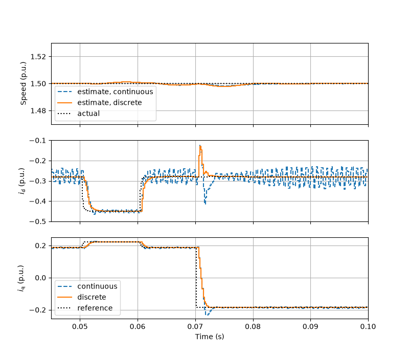
At this bandwidth, the continuous-time design is sensitive to the errors in the flux linkage map, resulting in poorly damped oscillations, while the discrete-time design remains well damped. In the largest steps, the voltage is limited.
References
Total running time of the script: (0 minutes 2.821 seconds)