2.2-kW IM, discrete-time current control

This example compares the continuous-time and direct discrete-time designs of the current controller in sensorless current-vector control of a 2.2-kW induction machine (IM). The sampling frequency is 5 kHz and the current-control bandwidth is 2π·700 rad/s, which is high compared with the sampling frequency.

from math import pi

import matplotlib.pyplot as plt

import motulator.drive.control.im as control
from motulator.drive import model, utils

Compute base values based on the nominal values.

nom = utils.NominalValues(U=400, I=5, f=50, P=2.2e3, tau=14.6)
base = utils.BaseValues.from_nominal(nom, n_p=2)

Configure the machine parameters.

par = model.InductionMachineInvGammaPars(
    n_p=2, R_s=3.7, R_R=2.1, L_sgm=0.021, L_M=0.224
)
est_par = control.InductionMachineInvGammaPars(
    n_p=2, R_s=3.7, R_R=2.1, L_sgm=0.021, L_M=0.224
)

Simulate the drive in torque-control mode at the constant speed of 0.5 p.u. The discrete-time design compensates for the delays itself, which is taken into account in the PWM configuration.

def simulate(discrete: bool):
    mdl = model.Drive(
        model.InductionMachine(par),
        model.ExternalRotorSpeed(),
        model.VoltageSourceConverter(u_dc=540),
        pwm=True,
    )
    mdl.mechanics.set_external_rotor_speed(lambda t: 0.5 * base.w_M)
    cfg = control.CurrentVectorControllerCfg(
        psi_s_nom=base.psi,
        i_s_max=2 * base.i,
        alpha_c=2 * pi * 700,
        T_s=200e-6,
        discrete=discrete,
    )
    pwm = control.PWM(k_comp=0) if discrete else None
    vector_ctrl = control.CurrentVectorController(est_par, cfg)
    vector_ctrl.observer.speed_observer.w_M = 0.5 * base.w_M  # Initial speed estimate
    ctrl = control.VectorControlSystem(vector_ctrl, pwm=pwm)
    ctrl.set_torque_ref(
        lambda t: nom.tau * (0.3 * (t > 0.3) + 0.2 * (t > 0.32) - 0.8 * (t > 0.34))
    )
    return model.Simulation(mdl, ctrl).simulate(t_stop=0.37)


res_cont, res_disc = simulate(discrete=False), simulate(discrete=True)

Plot the current responses in per-unit values.

_, (ax1, ax2) = plt.subplots(2, 1, figsize=(8, 5), sharex=True)
for res, ls, label in [(res_cont, "--", "continuous"), (res_disc, "-", "discrete")]:
    t, i_s = res.ctrl.t, res.ctrl.fbk.i_s / base.i
    ax1.plot(t, i_s.real, ls, ds="steps-post", label=label)
    ax2.plot(t, i_s.imag, ls, ds="steps-post", label=label)
i_s_ref = res_disc.ctrl.ref.i_s / base.i
ax1.plot(t, i_s_ref.real, "k:", ds="steps-post", label="reference")
ax2.plot(t, i_s_ref.imag, "k:", ds="steps-post", label="reference")
ax1.set_ylabel(r"$i_\mathrm{d}$ (p.u.)")
ax1.set_ylim(0.5, 0.7)
ax2.set_ylabel(r"$i_\mathrm{q}$ (p.u.)")
ax2.set_xlabel("Time (s)")
ax2.set_xlim(0.29, 0.37)
ax2.legend(loc="lower left")
for ax in (ax1, ax2):
    ax.grid(True)
plt.show()

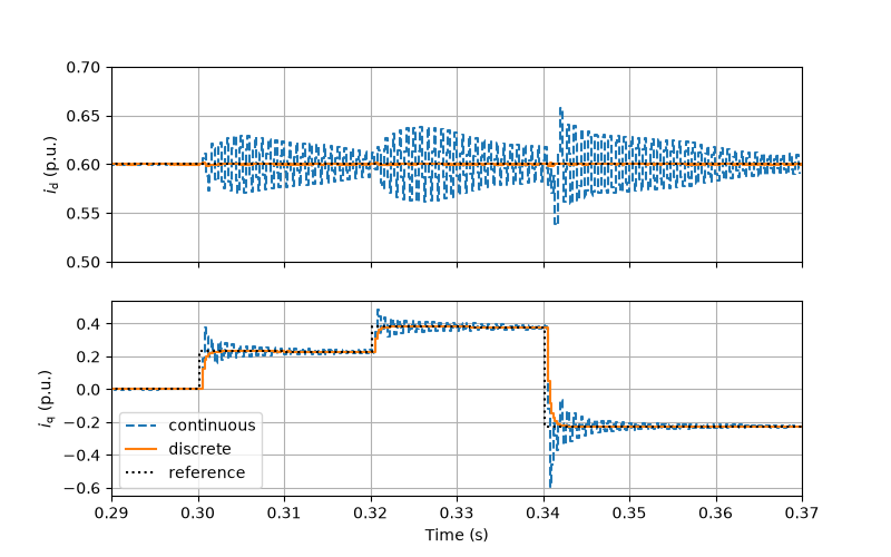
At this bandwidth, the continuous-time design results in poorly damped oscillations, while the discrete-time design is well damped.