2.2-kW IPMSM, active front end, CVC

This example simulates a 2.2-kW interior permanent-magnet synchronous machine (IPMSM) drive equipped with an active front end (AFE), i.e., a grid-connected converter that controls the DC-bus voltage. The machine-side converter uses sensorless current-vector control (CVC), and the grid-side converter uses grid-following current-vector control with a DC-bus voltage controller. The two control systems are independent: they have different sampling periods, and their carriers are not synchronized.

from math import pi

import matplotlib.pyplot as plt

import motulator.drive.control.sm as sm_control
from motulator.common.utils import complex2abc
from motulator.drive import model as drive_model
from motulator.drive import utils as drive_utils
from motulator.grid import control as grid_control
from motulator.grid import model as grid_model
from motulator.grid import utils as grid_utils

Compute base values based on the nominal values of the machine and the grid converter.

nom_m = drive_utils.NominalValues(U=370, I=4.3, f=75, P=2.2e3, tau=14)
base_m = drive_utils.BaseValues.from_nominal(nom_m, n_p=3)
nom_g = grid_utils.NominalValues(U=400, I=5, f=50, P=2.2e3)
base_g = grid_utils.BaseValues.from_nominal(nom_g)

Configure the system model. The two converters are fed from the same DC bus. The grid-side converter system and the drive are modeled separately, each with its own PWM, and combined into a composite model.

afe = grid_model.VoltageSourceConverter()
inv = drive_model.VoltageSourceConverter()
dc_bus = drive_model.DCBus(C_dc=470e-6, u_dc=650, converters=[afe, inv])

ac_filter = grid_model.LFilter(L_f=0.1 * base_g.L)
ac_source = grid_model.ThreePhaseSource(w_g=base_g.w, e_g=base_g.u)
grid_sys = grid_model.GridConverterSystem(
    afe, ac_filter, ac_source, pwm=True, dc_bus=dc_bus
)

par = drive_model.SynchronousMachinePars(
    n_p=3, R_s=3.6, L_d=0.036, L_q=0.051, psi_f=0.545
)
machine = drive_model.SynchronousMachine(par)
mechanics = drive_model.MechanicalSystem(J=0.015)
drive_sys = drive_model.Drive(machine, mechanics, inv, pwm=True, dc_bus=dc_bus)

mdl = drive_model.CompositeModel({"grid": grid_sys, "drive": drive_sys})

Configure the control systems. The grid-side control runs at 10 kHz (5-kHz switching frequency) and the machine-side control at 8 kHz (4-kHz switching frequency).

cfg_g = grid_control.CurrentVectorControllerCfg(
    i_max=1.5 * base_g.i, L=0.1 * base_g.L, T_s=100e-6
)
dc_bus_voltage_ctrl = grid_control.DCBusVoltageController(
    C_dc=470e-6, alpha_dc=2 * pi * 50, p_max=1.5 * base_g.p
)
ctrl_g = grid_control.GridConverterControlSystem(
    grid_control.CurrentVectorController(cfg_g), dc_bus_voltage_ctrl
)

est_par = par  # Assume accurate model parameter estimates
cfg_m = sm_control.CurrentVectorControllerCfg(
    i_s_max=1.5 * base_m.i, alpha_o=2 * pi * 100, T_s=125e-6
)
vector_ctrl = sm_control.CurrentVectorController(est_par, cfg_m)
speed_ctrl = sm_control.SpeedController(J=0.015, alpha_s=2 * pi * 4)
ctrl_m = sm_control.VectorControlSystem(vector_ctrl, speed_ctrl)

Set the references and the external load torque. The speed is reversed under load, after which the drive regenerates power to the grid.

ctrl_g.set_dc_bus_voltage_ref(650)
ctrl_g.set_reactive_power_ref(0)
ctrl_m.set_speed_ref(lambda t: (t > 0.1) * base_m.w_M - (t > 0.7) * 2 * base_m.w_M)
mechanics.set_external_load_torque(lambda t: (t > 0.4) * nom_m.tau)

Create the simulation object and simulate. The clocks of the two control systems are not synchronized: the machine-side control starts 40 µs after the grid-side control. The results of each model and its control system are available by the model names.

sim = drive_model.Simulation(
    mdl, {"grid": ctrl_g, "drive": ctrl_m}, t_start={"drive": 40e-6}
)
res = sim.simulate(t_stop=1)
res_drive = drive_model.SimulationResults(res.mdl.drive, res.ctrl.drive)
res_grid = grid_model.SimulationResults(res.mdl.grid, res.ctrl.grid)

Plot the drive and grid-side results in per-unit values.

# sphinx_gallery_thumbnail_number = 3
drive_utils.plot(res_drive, base_m)
grid_utils.plot_control_signals(res_grid, base_g)

• 
• 

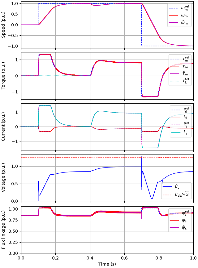
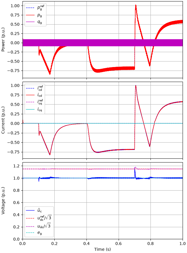
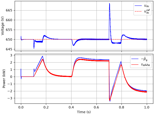
Plot the DC-bus voltage and the power balance: the power drawn from the grid (as estimated by the grid-side control) equals the mechanical power plus the losses (mainly the stator resistive losses), except during the DC-bus voltage transients.

p_g = res.ctrl.grid.fbk.p_g
p_M = res.mdl.drive.machine.tau_M * res.mdl.drive.machine.w_M
fig, (ax1, ax2) = plt.subplots(2, 1, sharex=True)
ax1.plot(res.mdl.t, res.mdl.drive.dc_bus.u_dc, label=r"$u_\mathrm{dc}$")
ax1.plot(
    res.ctrl.grid.t,
    res.ctrl.grid.ref.u_dc,
    "--",
    ds="steps-post",
    label=r"$u_\mathrm{dc}^\mathrm{ref}$",
)
ax1.set_ylabel("Voltage (V)")
ax1.legend()
ax2.plot(res.ctrl.grid.t, -p_g / 1e3, ds="steps-post", label=r"$-\hat{p}_\mathrm{g}$")
ax2.plot(res.mdl.t, p_M / 1e3, label=r"$\tau_\mathrm{M}\omega_\mathrm{M}$")
ax2.set_ylabel("Power (kW)")
ax2.set_xlabel("Time (s)")
ax2.legend()
plt.show()

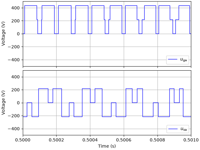
Plot the switched phase-a voltages of the two converters over one millisecond. The switching periods differ, and the switching instants are not aligned.

u_ga = complex2abc(res.mdl.grid.converter.u_c_ab)[0]
u_sa = complex2abc(res.mdl.drive.converter.u_c_ab)[0]
fig, (ax1, ax2) = plt.subplots(2, 1, sharex=True, sharey=True)
ax1.plot(res.mdl.t, u_ga, label=r"$u_\mathrm{ga}$")
ax1.set_ylabel("Voltage (V)")
ax1.legend(loc="lower right")
ax2.plot(res.mdl.t, u_sa, label=r"$u_\mathrm{sa}$")
ax2.set_ylabel("Voltage (V)")
ax2.set_xlabel("Time (s)")
ax2.set_xlim(0.5, 0.501)
ax2.set_ylim(-500, 500)
ax2.legend(loc="lower right")
plt.show()