Note
Go to the end to download the full example code.
2.2-kW IPMSM, dual-voltage-forming AFE, CVC#
This example simulates a 2.2-kW interior permanent-magnet synchronous machine (IPMSM) drive whose active front end (AFE) uses dual-voltage-forming control [1] and is connected to a weak grid. The grid-side converter regulates both the DC-bus voltage and its output voltage magnitude without a cascaded DC-bus voltage controller: the external power fed to the DC bus by the drive is estimated by a disturbance observer and fed forward. The machine-side converter uses sensorless current-vector control (CVC). The two control systems are independent: they have different sampling periods, and their carriers are not synchronized. The system model is otherwise the same as in 2.2-kW IPMSM, active front end, CVC, except for the weak grid.
from math import pi

import matplotlib.pyplot as plt

import motulator.drive.control.sm as sm_control
from motulator.drive import model as drive_model
from motulator.drive import utils as drive_utils
from motulator.grid import control as grid_control
from motulator.grid import model as grid_model
from motulator.grid import utils as grid_utils
Compute base values based on the nominal values of the machine and the grid converter.
nom_m = drive_utils.NominalValues(U=370, I=4.3, f=75, P=2.2e3, tau=14)
base_m = drive_utils.BaseValues.from_nominal(nom_m, n_p=3)
nom_g = grid_utils.NominalValues(U=400, I=5, f=50, P=2.2e3)
base_g = grid_utils.BaseValues.from_nominal(nom_g)
Configure the system model. The two converters are fed from the same DC bus. The grid is weak: its inductance is 0.74 p.u.
afe = grid_model.VoltageSourceConverter()
inv = drive_model.VoltageSourceConverter()
dc_bus = drive_model.DCBus(C_dc=470e-6, u_dc=650, converters=[afe, inv])

ac_filter = grid_model.LFilter(
    L_f=0.15 * base_g.L, R_f=0.05 * base_g.Z, L_g=0.74 * base_g.L
)
ac_source = grid_model.ThreePhaseSource(w_g=base_g.w, e_g=base_g.u)
grid_sys = grid_model.GridConverterSystem(
    afe, ac_filter, ac_source, pwm=True, dc_bus=dc_bus
)

par = drive_model.SynchronousMachinePars(
    n_p=3, R_s=3.6, L_d=0.036, L_q=0.051, psi_f=0.545
)
machine = drive_model.SynchronousMachine(par)
mechanics = drive_model.MechanicalSystem(J=0.015)
drive_sys = drive_model.Drive(machine, mechanics, inv, pwm=True, dc_bus=dc_bus)

mdl = drive_model.CompositeModel({"grid": grid_sys, "drive": drive_sys})
Configure the control systems. The grid-side control runs at 10 kHz (5-kHz switching frequency) and the machine-side control at 8 kHz (4-kHz switching frequency). The gains of the dual-voltage-forming controller are given in per-unit values of the grid converter [1].
cfg_g = grid_control.DualVoltageFormingControllerCfg(
    i_max=1.5 * base_g.i,
    L=0.3 * base_g.L,
    C_dc=470e-6,
    R=0.05 * base_g.Z,
    k_d=base_g.u / base_g.p,
    alpha_dc=0.15 * base_g.w,
    alpha_o=2 * base_g.w,
    alpha_o_dc=1.2 * base_g.w,
    k_v=6,
    alpha_c=6 * base_g.w,
    u_nom=base_g.u,
    w_nom=base_g.w,
    T_s=100e-6,
)
ctrl_g = grid_control.GridConverterControlSystem(
    grid_control.DualVoltageFormingController(cfg_g)
)

est_par = par  # Assume accurate model parameter estimates
cfg_m = sm_control.CurrentVectorControllerCfg(
    i_s_max=1.5 * base_m.i, alpha_o=2 * pi * 100, T_s=125e-6
)
vector_ctrl = sm_control.CurrentVectorController(est_par, cfg_m)
speed_ctrl = sm_control.SpeedController(J=0.015, alpha_s=2 * pi * 4)
ctrl_m = sm_control.VectorControlSystem(vector_ctrl, speed_ctrl)
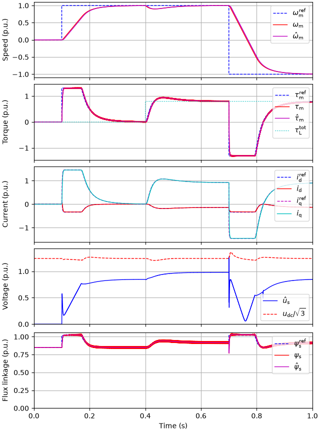
Set the references and the external load torque. The speed is reversed under load, after which the drive regenerates power to the grid.
ctrl_g.set_dc_bus_voltage_ref(650)
ctrl_g.set_ac_voltage_ref(base_g.u)
ctrl_m.set_speed_ref(lambda t: (t > 0.1) * base_m.w_M - (t > 0.7) * 2 * base_m.w_M)
mechanics.set_external_load_torque(lambda t: (t > 0.4) * nom_m.tau)
Create the simulation object and simulate. The clocks of the two control systems are not synchronized: the machine-side control starts 40 µs after the grid-side control. The results of each model and its control system are available by the model names.
sim = drive_model.Simulation(
    mdl, {"grid": ctrl_g, "drive": ctrl_m}, t_start={"drive": 40e-6}
)
res = sim.simulate(t_stop=1)
res_drive = drive_model.SimulationResults(res.mdl.drive, res.ctrl.drive)
res_grid = grid_model.SimulationResults(res.mdl.grid, res.ctrl.grid)
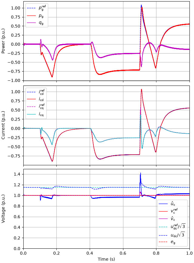
Plot the drive and grid-side results in per-unit values. The active power reference shown is the equivalent reference formed by the dual-voltage-forming controller from the estimated external power and the DC-bus energy error.
# sphinx_gallery_thumbnail_number = 3
drive_utils.plot(res_drive, base_m)
grid_utils.plot_control_signals(res_grid, base_g)
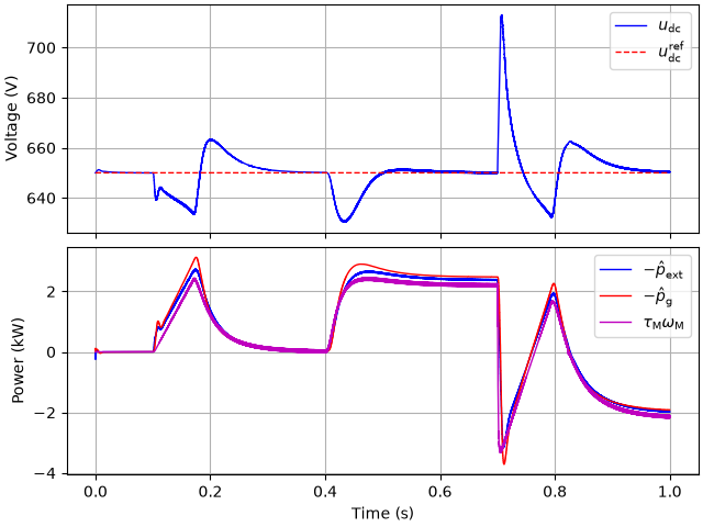
Plot the DC-bus voltage and the power balance: the estimated external power fed to the DC bus (the estimated disturbance power plus the grid power and the resistive losses of the filter) follows the mechanical power plus the losses (mainly the stator resistive losses), and the power drawn from the grid follows it with the delay of the current dynamics in the weak grid.
ctrl_ts = res.ctrl.grid
p_loss = 1.5 * cfg_g.R * abs(ctrl_ts.fbk.i_c) ** 2
p_ext = ctrl_ts.fbk.p_dis + ctrl_ts.fbk.p_g + p_loss
p_M = res.mdl.drive.machine.tau_M * res.mdl.drive.machine.w_M
fig, (ax1, ax2) = plt.subplots(2, 1, sharex=True)
ax1.plot(res.mdl.t, res.mdl.drive.dc_bus.u_dc, label=r"$u_\mathrm{dc}$")
ax1.plot(
    ctrl_ts.t,
    ctrl_ts.ref.u_dc,
    "--",
    ds="steps-post",
    label=r"$u_\mathrm{dc}^\mathrm{ref}$",
)
ax1.set_ylabel("Voltage (V)")
ax1.legend()
ax2.plot(ctrl_ts.t, -p_ext / 1e3, ds="steps-post", label=r"$-\hat{p}_\mathrm{ext}$")
ax2.plot(
    ctrl_ts.t, -ctrl_ts.fbk.p_g / 1e3, ds="steps-post", label=r"$-\hat{p}_\mathrm{g}$"
)
ax2.plot(res.mdl.t, p_M / 1e3, label=r"$\tau_\mathrm{M}\omega_\mathrm{M}$")
ax2.set_ylabel("Power (kW)")
ax2.set_xlabel("Time (s)")
ax2.legend()
plt.show()
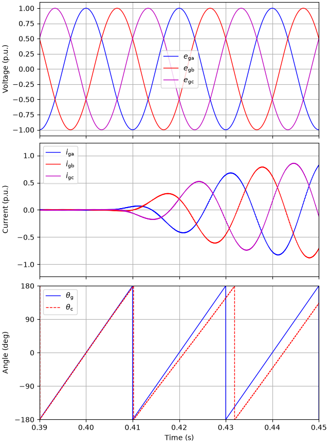
Plot the grid-side waveforms around the load torque step. The converter current increases within a few milliseconds, as the estimated external power is fed forward.
grid_utils.plot_grid_waveforms(
    res_grid, base_g, t_lims=(0.39, 0.45), plot_pcc_voltage=False
)
References
Total running time of the script: (0 minutes 21.239 seconds)