5.6-kW deep-bar IM, direct-on-line start#

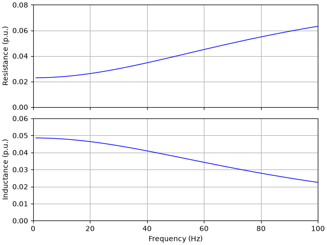
This example simulates the direct-on-line start of a 5.6-kW induction machine (IM) with deep rotor bars. At high slip frequencies, the eddy currents in the bars increase the rotor resistance and decrease the rotor leakage inductance (deep-bar effect), which increases the starting torque. The deep-bar effect is modeled by means of the cage impedance [1], and the main-flux saturation is also included. The parameters of the machine are given in [2].

from math import pi

import matplotlib.pyplot as plt
import numpy as np

from motulator.common.utils import set_style
from motulator.drive import model, utils

Compute base values based on the nominal values. The nominal speed is 1770 r/min.

nom = utils.NominalValues(U=460, I=9.5, f=60, P=5.6e3, tau=5.6e3 / (2 * pi * 1770 / 60))
base = utils.BaseValues.from_nominal(nom, n_p=2)

The Γ model is used, with a constant leakage inductance and a stator inductance that saturates as a function of the stator flux linkage magnitude.

def L_s(psi, L_su=0.1857, c=1.4, S=6):
    """Stator inductance (H) as a function of the flux linkage magnitude (Vs)."""
    return L_su / (1 + (psi / c) ** S)

The cage impedance is a ladder circuit of the first order, whose DC resistance is 0.64 Ω and DC inductance is 3.6 mH. Its resistance increases and its inductance decreases with the frequency of the rotor current, i.e., with the slip frequency.

cage = model.CageImpedance(R=[0.64, 2.1], L=[3.6e-3])

f = np.linspace(1, 100, 100)
Z_c = cage.Z(2j * pi * f)

set_style()
fig, (ax1, ax2) = plt.subplots(2, 1, sharex=True)
ax1.plot(f, np.real(Z_c) / base.Z)
ax1.set_ylabel("Resistance (p.u.)")
ax1.set_ylim(0, 0.08)
ax2.plot(f, np.imag(Z_c) / (2 * pi * f) / base.L)
ax2.set_ylabel("Inductance (p.u.)")
ax2.set_ylim(0, 0.06)
ax2.set_xlabel("Frequency (Hz)")
ax2.set_xlim(0, 100)
plt.show()

Configure the system model. For comparison, the machine can also be modeled without the deep-bar effect, in which case the rotor resistance is the DC resistance of the cage and the leakage inductance includes the DC inductance of the cage. The machine drives a fan, whose load torque is proportional to the square of the speed.

def create_model(deep_bars: bool) -> model.GridConnectedMachine:
    """Create the model of the grid-connected machine."""
    if deep_bars:
        R_r, L_ell = cage, 12.4e-3
    else:
        R_r, L_ell = 0.64, 12.4e-3 + 3.6e-3
    par = model.InductionMachinePars(n_p=2, R_s=0.93, R_r=R_r, L_ell=L_ell, L_s=L_s)
    machine = model.InductionMachine(par)
    k = nom.tau / base.w_M**2  # Quadratic load torque profile
    mechanics = model.MechanicalSystem(J=0.1, B_L=lambda w_M: k * abs(w_M))
    ac_source = model.ThreePhaseSource(w_g=base.w, e_g=base.u)
    return model.GridConnectedMachine(machine, mechanics, ac_source)

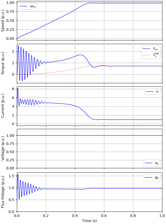
Simulate the start with the deep-bar effect and plot the results in per-unit values. After the start, the machine operates close to its nominal operating point.

sim = model.Simulation(create_model(deep_bars=True))
res = sim.simulate(t_stop=1)
utils.plot(res, base)

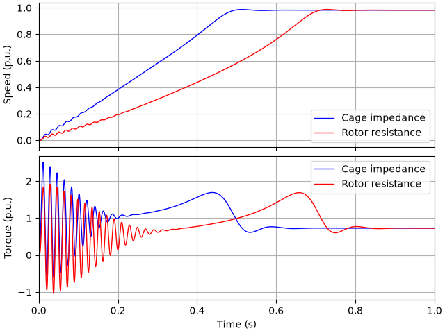
Simulate the start without the deep-bar effect and compare the results. The deep-bar effect increases the torque during the start, while the operation at low slip frequencies is not affected.

sim = model.Simulation(create_model(deep_bars=False))
res_ref = sim.simulate(t_stop=1)

fig, (ax1, ax2) = plt.subplots(2, 1, sharex=True)
for r, label in ((res, "Cage impedance"), (res_ref, "Rotor resistance")):
    ax1.plot(r.mdl.t, r.mdl.machine.w_M / base.w_M, label=label)
    ax2.plot(r.mdl.t, r.mdl.machine.tau_M / base.tau, label=label)
ax1.set_ylabel("Speed (p.u.)")
ax1.legend(loc="lower right")
ax2.set_ylabel("Torque (p.u.)")
ax2.legend(loc="upper right")
ax2.set_xlabel("Time (s)")
ax2.set_xlim(0, 1)
plt.show()

# sphinx_gallery_thumbnail_number = 3

References

Total running time of the script: (0 minutes 3.313 seconds)

Gallery generated by Sphinx-Gallery